GC-IRMS data processing example: carbon

carbon isotopes in alkanes

2021-11-04

Introduction

This is an example of a data processing pipeline for compound-specific Gas Chromatography Isotope Ratio Mass Spectrometry (GC-IRMS) carbon isotope measurements. It can be downloaded as a template (or just to see the plain-text code) by following the Source link above. Knitting for stand-alone data analysis works best to HTML rather than the website rendering you see here. To make this formatting change simply delete line #6 in the template file (the line that says rmarkdown::html_vignette:).

Note that all code chunks that contain a critical step towards the final data (i.e. do more than visualization or a data summary) are marked with (*) in the header to make it easier to follow all key steps during interactive use.

This example was run using isoreader version 1.3.1 and isoprocessor version 0.6.11. If you want to reproduce the example, please make sure that you have these or newer versions of both packages installed:

# restart your R session (this command only works in RStudio)
.rs.restartR()

# installs the development tools package if not yet installed
if(!requireNamespace("devtools", quietly = TRUE)) install.packages("devtools") 

# installs the newest version of isoreader and isoprocessor
devtools::install_github("isoverse/isoreader")
devtools::install_github("isoverse/isoprocessor")

Load packages

library(tidyverse) # general data wrangling and plotting
library(isoreader) # reading the raw data files
library(isoprocessor) # processing the data

This analysis was run using isoreader version 1.3.1 and isoprocessor version 0.6.11.

For use as a data processing template, please follow the Source link above, download the raw file and adapt as needed. Knitting for stand-alone data analysis works best to HTML rather than the in-package default html_vignette.

All code chunks that contain a critical step towards the final data (i.e. do more than visualization or a data summary) are marked with (*) in the header to make it easier to follow all key steps during interactive use.

Load data

Read raw data files (*)

# set file path(s) to data files, folders or rds collections 
# can be multiple folders or mix of folders and files, using example data set here
# (this is a reduced data set of mostly standards with just a few example samples)
data_path <- iso_get_processor_example("gc_irms_example_carbon.cf.rds")

# read files
iso_files_raw <- 
  # path to data files
  data_path %>% 
  # read data files in parallel for fast read
  iso_read_continuous_flow(parallel = TRUE) %>%
  # filter out files with read errors (e.g. from aborted analysis)
  iso_filter_files_with_problems()
#> Info: preparing to read 1 data files (all will be cached), setting up 1 par...
#> Process 1: reading file 'gc_irms_example_carbon.cf.rds' with '.cf.rds' read...
#> Process 1: loaded 45 data files from R Data Storage
#> Info: finished reading 1 files in 2.89 secs
#> Info: removing 0/45 files that have any error (keeping 45)

Process file info & peak table (*)

# process
iso_files <- iso_files_raw %>% 
  # set peak table from vendor data table
  iso_set_peak_table_automatically_from_vendor_data_table() %>% 
  # convert units from mV to V for amplitudes and area
  iso_convert_peak_table_units(V = mV, Vs = mVs) %>% 
  # rename key file info columns
  iso_rename_file_info(id1 = `Identifier 1`, id2 = `Identifier 2`) %>% 
  # parse text info into numbers
  iso_parse_file_info(number = Analysis) %>% 
  # process other file information that is specific to the naming conventions
  # of this particular sequence
  iso_mutate_file_info(
    # what is the type of each analysis?
    type = case_when(
      str_detect(id1, "[Zz]ero")      ~ "on_off",
      str_detect(id1, "[Ll]inearity") ~ "lin",
      str_detect(id1, "A5")           ~ "std",
      TRUE                            ~ "sample"
    ),
    # was there seed oxidation?
    seed_oxidation = ifelse(`Seed Oxidation` == "1", "yes", "no"),
    # what was the injection volume based on the AS method name?
    injection_volume = str_extract(`AS Method`, "AS PTV [0-9.]+") %>% 
      parse_number() %>% iso_double_with_units("uL"),
    # what was the concentration? (assuming Preparation = concentration or volume)
    concentration = str_extract(Preparation, "[0-9.]+ ?ng( per |/)uL") %>% 
      parse_number() %>% iso_double_with_units("ng/uL"),
    # or the volume?
    volume = str_extract(Preparation, "[0-9.]+ ?uL") %>% 
      parse_number() %>% iso_double_with_units("uL"),
    # what folder are the data files in? (assuming folder = sequence)
    folder = basename(dirname(file_path))
  ) %>% 
  # add in additional sample metadata (could be any info)
  # note: this would typically be stored in / read from a csv or excel file
  iso_add_file_info(
    tibble::tribble(
      # column names
      ~id1,                           ~sample,          ~fraction,
      # metadata (row-by-row)
      "OG268_CZO-SJER_F1",            "SJER",           "F1",
      "OG271_CZO-CTNA_F1",            "CTNA",           "F1",
      "OG281_CZO-Niwot_Tundra2_F1",   "Niwot_Tundra2",  "F1",
      "OG282_CZO-Niwot_Tundra1_F1",   "Niwot_Tundra1",  "F1"
    ),
    join_by = "id1"
  ) %>% 
  # focus only on the relevant file info, discarding the rest
  iso_select_file_info(
    folder, Analysis, file_datetime, id1, id2, type, sample, 
    seed_oxidation, injection_volume, concentration, volume
  )
#> Info: setting peak table for 45 file(s) from vendor data table with the following renames:
#> - for 45 file(s): 'Nr.'->'peak_nr', 'Is Ref.?'->'is_ref', 'Start'->'rt_start', 'Rt'->'rt', 'End'->'rt_end', 'Ampl 44'->'amp44', 'Ampl 45'->'amp45', 'Ampl 46'->'amp46', 'BGD 44'->'bgrd44_start', 'BGD 45'->'bgrd45_start', 'BGD 46'->'bgrd46_start', 'BGD 44'->'bgrd44_end', 'BGD 45'->'bgrd45_end', 'BGD 46'->'bgrd46_end', 'rIntensity 44'->'area44', 'rIntensity 45'->'area45', 'rIntensity 46'->'area46', 'rR 45CO2/44CO2'->'r45/44', 'rR 46CO2/44CO2'->'r46/44', 'rd 45CO2/44CO2'->'rd45/44', 'rd 46CO2/44CO2'->'rd46/44', 'd 45CO2/44CO2'->'d45/44', 'd 46CO2/44CO2'->'d46/44', 'd 13C/12C'->'d13C', 'd 18O/16O'->'d18O', 'd 17O/16O'->'d17O', 'AT% 13C/12C'->'at13C', 'AT% 18O/16O'->'at18O'
#> Info: converting peak table column units where applicable from 'mV'->'V' and 'mVs'->'Vs' for columns matching 'everything()'
#> Info: renaming the following file info across 45 data file(s): 'Identifier 1'->'id1', 'Identifier 2'->'id2'
#> Info: parsing 1 file info columns for 45 data file(s):
#>  - to number: 'Analysis'
#> Info: mutating file info for 45 data file(s)
#> Info: adding new file information ('sample', 'fraction') to 45 data file(s), joining by 'id1'...
#>  - 'id1' join: 4/4 new info rows matched 4/45 data files
#> Info: selecting/renaming the following file info across 45 data file(s): 'folder', 'Analysis', 'file_datetime', 'id1', 'id2', 'type', 'sample', 'seed_oxidation', 'injection_volume', 'concentration', 'volume'

Show file information

# display file information
iso_files %>% 
  iso_get_file_info() %>% select(-file_id, -folder) %>% 
  iso_make_units_explicit() %>% knitr::kable()
#> Info: aggregating file info from 45 data file(s)

Analysis	file_datetime	id1	id2	type	sample	seed_oxidation	injection_volume [uL]	concentration [ng/uL]	volume [uL]
2026	2017-10-26 02:22:23	CO2 zero	6V	on_off	NA	no	NA	NA	NA
2030	2017-10-26 02:55:44	Linearity CO2	NA	lin	NA	no	NA	NA	NA
2034	2017-10-26 09:15:48	A5	0.5ul	std	NA	yes	0.5	14	NA
2041	2017-10-26 20:50:38	A5	3ul	std	NA	no	3.0	14	NA
2047	2017-10-27 05:50:04	A5	3ul	std	NA	yes	3.0	14	NA
2061	2017-10-28 01:29:27	OG271_CZO-CTNA_F1	1.5uL	sample	CTNA	yes	1.5	NA	25
2093	2017-10-30 00:32:04	A5	0.5ul	std	NA	yes	0.5	14	NA
2099	2017-10-30 10:33:19	A5	0.5ul	std	NA	yes	0.5	14	NA
2106	2017-10-30 22:25:45	OG281_CZO-Niwot_Tundra2_F1	1.5uL	sample	Niwot_Tundra2	yes	1.5	NA	150
2114	2017-10-31 10:08:42	A5	1.5ul	std	NA	yes	1.5	14	NA
2132	2017-11-01 18:33:25	A5 conc	1ul	std	NA	yes	1.0	140	NA
2138	2017-11-02 07:48:12	A5 conc	1.5ul	std	NA	yes	1.5	140	NA
2027	2017-10-26 02:30:42	CO2 zero	3V	on_off	NA	no	NA	NA	NA
2031	2017-10-26 04:30:54	A5	0.5ul	std	NA	yes	0.5	14	NA
2035	2017-10-26 10:50:43	A5	1.5ul	std	NA	yes	1.5	14	NA
2044	2017-10-27 00:23:25	A5	4.5ul	std	NA	no	4.5	14	NA
2053	2017-10-27 14:49:22	OG268_CZO-SJER_F1	1.5uL	sample	SJER	yes	1.5	NA	50
2069	2017-10-28 12:37:31	A5	1.5ul	std	NA	yes	1.5	14	NA
2096	2017-10-30 05:48:23	A5	1.5ul	std	NA	yes	1.5	14	NA
2100	2017-10-30 12:08:16	A5	1.5ul	std	NA	yes	1.5	14	NA
2107	2017-10-31 00:00:40	OG282_CZO-Niwot_Tundra1_F1	1.5uL	sample	Niwot_Tundra1	yes	1.5	NA	150
2115	2017-10-31 11:43:46	A5	3ul	std	NA	yes	3.0	14	NA
2139	2017-11-02 15:13:36	A5 conc	1ul	std	NA	yes	1.0	140	NA
2028	2017-10-26 02:39:02	CO2 zero	1.2V	on_off	NA	no	NA	NA	NA
2032	2017-10-26 06:05:49	A5	1.5ul	std	NA	yes	1.5	14	NA
2036	2017-10-26 12:25:48	A5	3ul	std	NA	yes	3.0	14	NA
2045	2017-10-27 02:40:08	A5	0.5ul	std	NA	yes	0.5	14	NA
2056	2017-10-27 19:34:08	A5	1.5ul	std	NA	yes	1.5	14	NA
2075	2017-10-28 20:27:22	A5	1.5ul	std	NA	yes	1.5	14	NA
2097	2017-10-30 07:23:28	A5	3ul	std	NA	yes	3.0	14	NA
2101	2017-10-30 13:43:23	A5	3ul	std	NA	yes	3.0	14	NA
2116	2017-10-31 13:18:39	A5 conc	1ul	std	NA	yes	1.0	140	NA
2136	2017-11-02 04:38:25	A5 conc	0.5ul	std	NA	yes	0.5	140	NA
2140	2017-11-02 16:48:30	A5 conc	2ul	std	NA	yes	2.0	140	NA
2029	2017-10-26 02:47:22	CO2 zero	0.7V	on_off	NA	no	NA	NA	NA
2033	2017-10-26 07:40:55	A5	3ul	std	NA	yes	3.0	14	NA
2040	2017-10-26 19:07:47	A5	1.5ul	std	NA	yes	1.5	14	NA
2046	2017-10-27 04:15:02	A5	1.5ul	std	NA	yes	1.5	14	NA
2060	2017-10-27 23:54:33	A5 conc	1ul	std	NA	no	1.0	140	NA
2086	2017-10-29 13:58:06	A5	1.5ul	std	NA	yes	1.5	14	NA
2098	2017-10-30 08:58:24	A5 conc	1ul	std	NA	yes	1.0	140	NA
2102	2017-10-30 15:18:16	A5 conc	1ul	std	NA	yes	1.0	140	NA
2113	2017-10-31 08:33:47	A5	0.5ul	std	NA	yes	0.5	14	NA
2117	2017-10-31 14:53:43	A5 conc	3ul	std	NA	yes	3.0	140	NA
2137	2017-11-02 06:13:18	A5 conc	1ul	std	NA	yes	1.0	140	NA

Example chromatograms

# plot the chromatograms
iso_plot_continuous_flow_data(
  # select a few analyses (these #s must exist!)
  iso_filter_files(iso_files, Analysis %in% c(2046, 2106, 2107)),
  # select data and aesthetics
  data = c(44), color = id1, panel = Analysis,
  # zoom in on time interval
  time_interval = c(1000, 3200),
  # peak labels for all peaks > 2V
  peak_label = iso_format(rt, d13C, signif = 3),
  peak_label_options = list(size = 3),
  peak_label_filter = amp44 > 2000
) +
  # customize resulting ggplot
  theme(legend.position = "bottom")
#> Info: applying file filter, keeping 3 of 45 files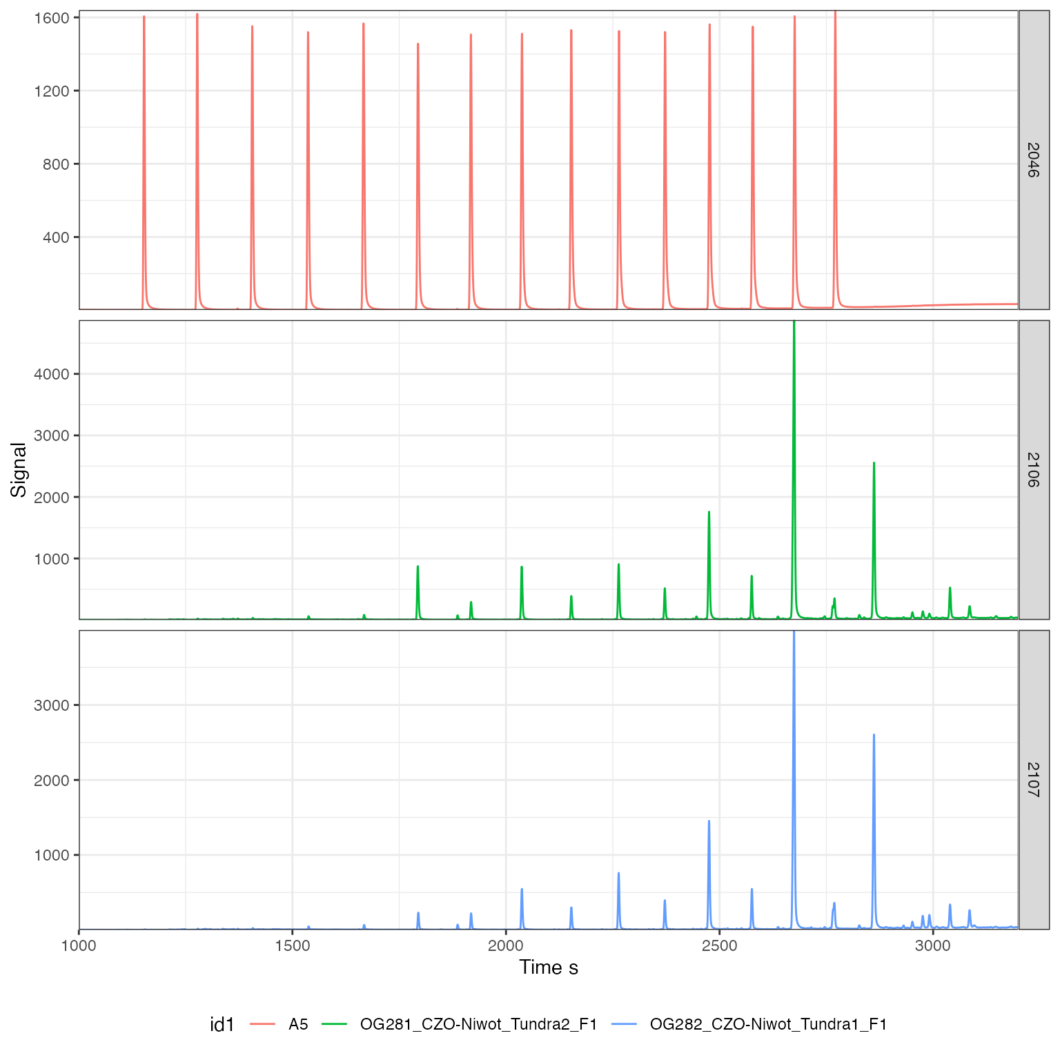

ON/OFFs

# find files with zero in the Identifier 1 field
on_offs <- iso_files %>% iso_filter_files(type == "on_off") 
#> Info: applying file filter, keeping 4 of 45 files

# visualize the on/offs  
iso_plot_continuous_flow_data(on_offs, data = 44, color = id2)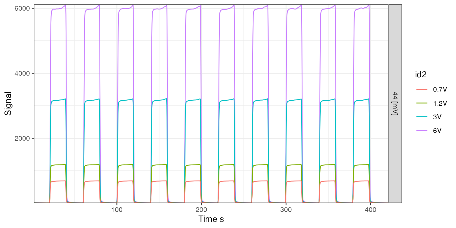

Summary

# calculate on/off summary
on_off_summary <- 
  on_offs %>% 
  # retrieve peak table
  iso_get_peak_table(
    select = c(amp44, area44, d13C),
    include_file_info = c(file_datetime, id2)
  ) %>% 
  # summarize information
  group_by(file_datetime, id2) %>% 
  iso_summarize_data_table() 
#> Info: aggregating peak table from 4 data file(s), including file info 'c(file_datetime, id2)'
  

# table
on_off_summary %>% iso_make_units_explicit() %>% knitr::kable(digits = 3)

file_datetime	id2	n	amp44 mean [V]	amp44 sd	area44 mean [Vs]	area44 sd	d13C mean [permil]	d13C sd
2017-10-26 02:22:23	6V	10	6.091	0.010	112.848	0.330	0.006	0.012
2017-10-26 02:30:42	3V	10	3.201	0.003	59.386	0.141	0.001	0.018
2017-10-26 02:39:02	1.2V	10	1.183	0.001	21.968	0.054	-0.006	0.024
2017-10-26 02:47:22	0.7V	10	0.681	0.001	12.638	0.030	-0.031	0.052

# plot
on_off_summary %>% 
  # use generic data plot function
  iso_plot_data(
    x = file_datetime, y = `d13C sd`,
    size = `amp44 mean`, color = id2,
    points = TRUE,
    date_labels = "%b %d - %H:%M"
  ) + 
  # customize resulting ggplot
  expand_limits(y = 0)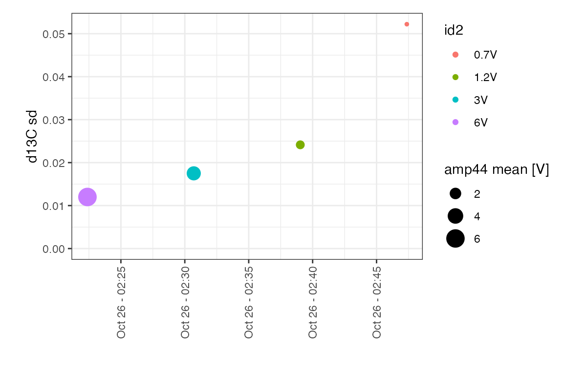 

Linearity

# find files with linearity in the Identifier 1 field
lins <- iso_files %>% iso_filter_files(type == "lin") 
#> Info: applying file filter, keeping 1 of 45 files

# visualize the linearity runs
iso_plot_continuous_flow_data(lins, data = 44, color = format(file_datetime))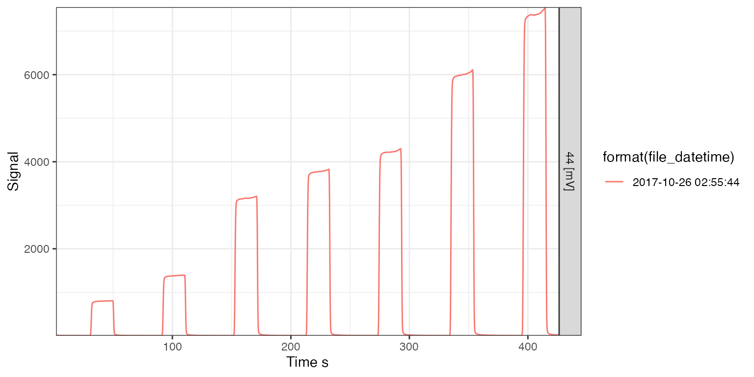

Summary

# calculate linearity summary
linearity_summary <- 
  lins %>% 
  # retrieve data table
  iso_get_peak_table(
    select = c(amp44, area44, d13C),
    include_file_info = c(file_datetime)
  ) %>% 
  # calculate linearity regression lines
  nest(data = -file_datetime) %>% 
  mutate(
    fit = map(data, ~lm(d13C ~ amp44, data = iso_strip_units(.x))),
    coefs = map(fit, broom::tidy)
  )
#> Info: aggregating peak table from 1 data file(s), including file info 'c(file_datetime)'

# table
linearity_summary %>%
  unnest(coefs) %>%
  select(file_datetime, term, estimate, std.error) %>%
  filter(term == "amp44") %>%
  mutate(
    term = "linearity [permil/V]",
    estimate = signif(estimate, 2),
    std.error = signif(std.error, 1)
  ) %>% 
  knitr::kable(digits = 4)

file_datetime	term	estimate	std.error
2017-10-26 02:55:44	linearity [permil/V]	-0.017	0.001

# plot
linearity_summary %>% 
  unnest(data) %>% 
  # use generic data plot function
  iso_plot_data(
    x = amp44, y = d13C,
    color = format(file_datetime),
    points = TRUE,
    panel = file_datetime,
    geom_smooth(method = "lm")
  )
#> `geom_smooth()` using formula 'y ~ x'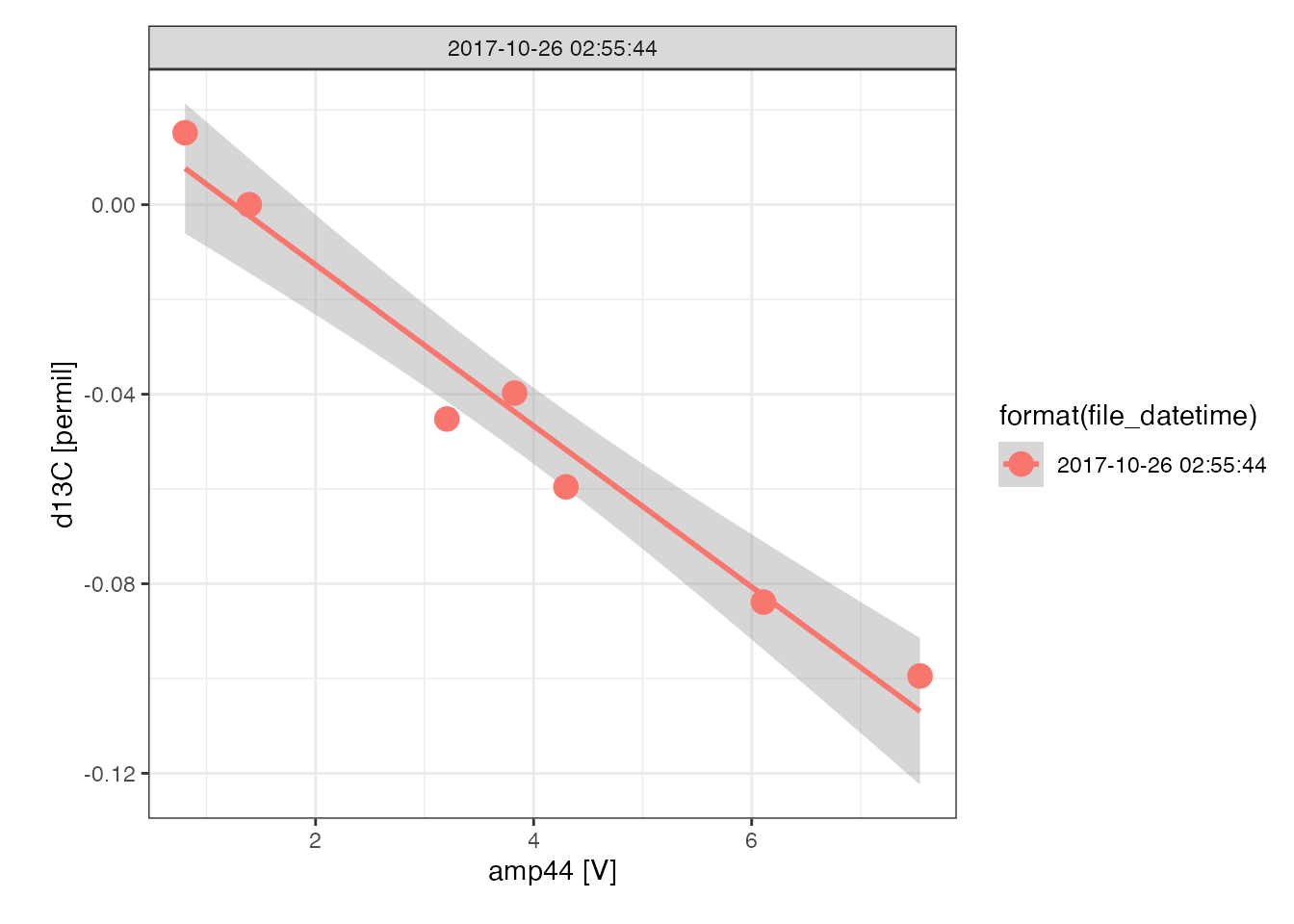

Samples and Standards

Load peak maps

# this information is often maintained in a csv or Excel file instead
# but generated here from scratch for demonstration purposes
peak_maps <- 
  tibble::tribble(
    # column names -> defining 2 peak maps, 'std' and 'sample' here
    # but could define an unlimited number of different maps
    ~compound, ~ref_nr, ~`rt:std`,  ~`rt:sample`,
    # peak map data (row-by-row)
    "CO2",          1,        79,                 79,
    "CO2",          2,      178,                178,
    "CO2",          3,      278,                278,
    "CO2",          4,      377,                377,
    "CO2",          5,      477,                477,
    "CO2",          6,      576,                576,
    "CO2",          7,      676,                676,
    "CO2",          8,      775,                775,
    "CO2",          9,      875,                875,
    "nC16",         NA,     1156,               1156,
    "nC17",         NA,     1280,               1280,
    "nC18",         NA,     1409,               1409,
    "nC19",         NA,     1540,               1540,
    "nC20",         NA,     1670,               1670,
    "nC21",         NA,     1797,               1797,
    "nC22",         NA,     1921,               1921,
    "nC23",         NA,     2040,               2040,
    "nC24",         NA,     2156,               2156,
    "nC25",         NA,     2267,               2267,
    "nC26",         NA,     2375,               2375,
    "nC27",         NA,     2479,               2479,
    "nC28",         NA,     2580,               2580,
    "nC29",         NA,     2674,               2678,
    "nC30",         NA,     2770,               2773,
    "nC31",         NA,     NA,               2863,
    "CO2",          10,     3552,               3552,
    "CO2",          11,     3592,               3592
  )
peak_maps %>% knitr::kable(digits = 0)

compound	ref_nr	rt:std	rt:sample
CO2	1	79	79
CO2	2	178	178
CO2	3	278	278
CO2	4	377	377
CO2	5	477	477
CO2	6	576	576
CO2	7	676	676
CO2	8	775	775
CO2	9	875	875
nC16	NA	1156	1156
nC17	NA	1280	1280
nC18	NA	1409	1409
nC19	NA	1540	1540
nC20	NA	1670	1670
nC21	NA	1797	1797
nC22	NA	1921	1921
nC23	NA	2040	2040
nC24	NA	2156	2156
nC25	NA	2267	2267
nC26	NA	2375	2375
nC27	NA	2479	2479
nC28	NA	2580	2580
nC29	NA	2674	2678
nC30	NA	2770	2773
nC31	NA	NA	2863
CO2	10	3552	3552
CO2	11	3592	3592

Fetch peak table (*)

# identify peaks
peak_table_w_ids <- iso_files %>% 
  # focus on standards and samples only
  iso_filter_files(type %in% c("std", "sample")) %>% 
  # filter out analyses that
  ## a) did not inject
  iso_filter_files(!Analysis %in% c(2031, 2040, 2069, 2098, 2116, 2138)) %>%
  ## b) had double or rogue peaks from mis-injection
  iso_filter_files(!Analysis %in% c(2044, 2132, 2134)) %>% 
  # map peaks
  iso_map_peaks(peak_maps, map_id = type) %>% 
  # peak table
  iso_get_peak_table(include_file_info = everything())
#> Info: applying file filter, keeping 40 of 45 files
#> Info: applying file filter, keeping 34 of 40 files
#> Info: applying file filter, keeping 32 of 34 files
#> Info: 829 of 973 peaks in 32 files were successfully mapped using 2 peak maps ('std', 'sample'). 144 peak(s) could not be mapped. 7 expected peak(s) are missing.
#> Info: aggregating peak table from 32 data file(s), including file info 'everything()'

Inspect peak mappings

# use same plotting as earlier, except now with peak features added in
iso_files %>% 
  iso_filter_files(Analysis %in% c(2046, 2106, 2107)) %>% 
  iso_plot_continuous_flow_data(
    # select data and aesthetics
    data = 44, color = id1, panel = Analysis,
    # zoom in on time interval
    time_interval = c(1000, 3200),
    # provide our peak table with ids
    peak_table = peak_table_w_ids, 
    # define peak labels, this can be any valid expression
    peak_label = iso_format(id = peak_info, d13C), 
    # specify which labels to show (removing the !is_identified or putting a 
    # restriction by retention time can help a lot with busy chromatograms)
    peak_label_filter = is_identified | !is_identified | is_missing
  )  +
  # customize resulting ggplot
  theme(legend.position = "bottom")
#> Info: applying file filter, keeping 3 of 45 files
#> Warning: ggrepel: 1 unlabeled data points (too many overlaps). Consider
#> increasing max.overlaps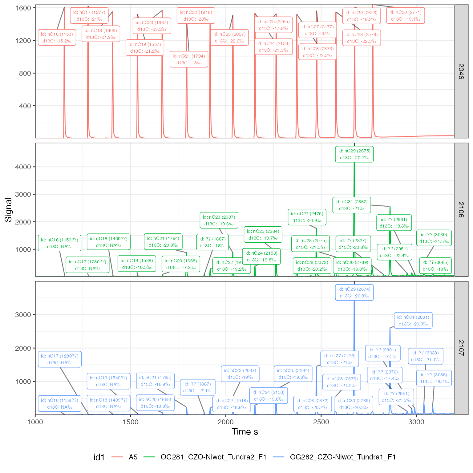

Overview of unclear peak mappings

# look at missing and unidentified peaks summary (not run during knitting)
# -> check if any of the missing peaks are unexpected (should be there but aren't)
# -> check if any unidentified peaks should be added to the peak maps
# -> check if any ambiguous peaks need clearer peak map retention times
# when in doubt, look at the chromatograms of the problematic files!
# as needed: iterate on peak map update, then peak mapping inspection
peak_table_w_ids %>% 
  iso_get_problematic_peak_mappings() %>% 
  iso_summarize_peak_mappings()

Reference peaks

# examine variation in the reference peaks
peak_table_w_ids %>% 
  # focus on reference peaks only
  filter(!is.na(ref_nr)) %>% 
  # mark ref peak used for raw delta values (assuming the same in all anlysis)
  mutate(
    ref_info = paste0(ref_nr, ifelse(is_ref == 1, "*", "")) %>% factor() %>% fct_inorder()
  ) %>% 
  # visualize
  iso_plot_ref_peaks(
    # specify the ratios to visualize
    x = Analysis, ratio = `r45/44`, fill = ref_info,
    panel_scales = "fixed"
  ) +
  labs(x = "Analysis", fill = "Reference\npeak")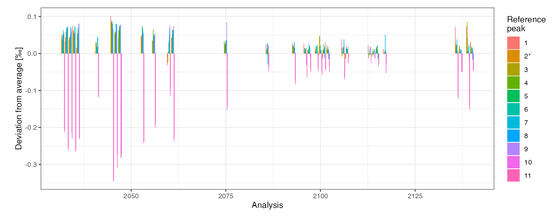

Analyte peaks

Select analyte peaks (*)

# focus on analyte peaks and calculate useful summary statistics
peak_table_analytes <- peak_table_w_ids %>% 
  # omit reference peaks for further processing (i.e. analyte peaks only)
  filter(is.na(ref_nr)) %>% 
  # for each analysis, calculate a few useful summary statistics
  iso_mutate_peak_table(
    group_by = file_id,
    rel_area = area44 / sum(area44, na.rm = TRUE),
    # calculate mean area for all peaks
    mean_area = mean(area44, na.rm = TRUE),
    # calculate mean area and amplitude for identified peaks
    mean_area_identified = mean(area44[!is.na(compound)], na.rm = TRUE),
    mean_amp_identified = mean(amp44[!is.na(compound)], na.rm = TRUE)
  )
#> Info: mutating peak table grouped by 'file_id', column(s) 'rel_area', 'mean_area', 'mean_area_identified', 'mean_amp_identified' added.

First look

peak_table_analytes %>% 
  # focus on identified peaks (comment out this line to see ALL peaks)
  filter(!is.na(compound)) %>% 
  # visualize with convenience function iso_plot_data
  iso_plot_data(
    # choose x and y (multiple y possible)
    x = area44, y = c(amp44, d13C),
    # choose aesthetics
    color = compound, shape = type, label = compound, size = 3,
    # decide what geoms to include
    points = TRUE
  ) +
  # further customize ggplot with a log scale x axis
  scale_x_log10()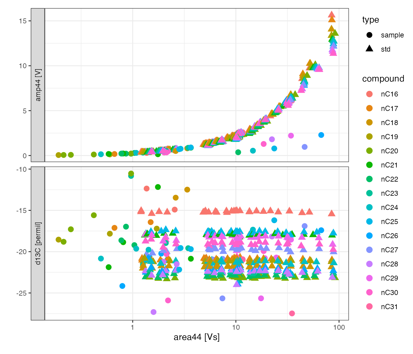

Optionally - use interactive plot

# optinally, use an interactive plot to explore your data
# - make sure you install the plotly library --> install.packages("plotly")
# - switch to eval=TRUE in the options of this chunk to include in knit
# - this should work for all plots in this example processing file
library(plotly)
ggplotly(dynamicTicks = TRUE)

Evaluate signal yield

# evaluate yield
# (only makes sense if both injection volume and concentration are available)
peak_table_analytes %>% 
  # focus on standards
  filter(type == "std") %>% 
  # calculate injection amount
  mutate(injection = iso_double_with_units(
    as.numeric(injection_volume) * as.numeric(concentration), units = "ng")) %>% 
  # visualize
  iso_plot_data(
    # x and y
    x = injection, y = c(mean_area_identified, mean_amp_identified),
    # aesthetics
    color = factor(injection_volume), shape = factor(concentration), 
    size = file_datetime,
    points = TRUE
  ) +
  # modify plot with trendline and axis limits
  geom_smooth(method = "lm", mapping = aes(color = NULL, shape = NULL)) +
  expand_limits(y = 0, x = 0)
#> `geom_smooth()` using formula 'y ~ x'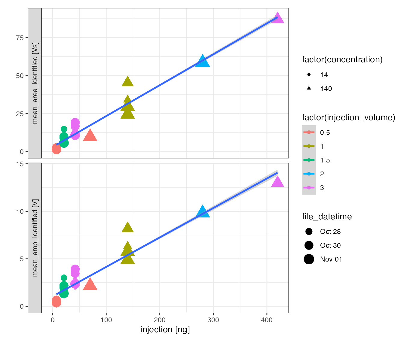

Isotope standard values

Load isotope standards

# this information is often maintained in a csv or Excel file instead
# but generated here from scratch for demonstration purposes
standards <- 
  tibble::tribble(
    ~compound,   ~true_d13C,
    "nC16",         -26.15,
    "nC17",         -31.88,
    "nC18",         -32.70,
    "nC19",         -31.99,
    "nC20",         -33.97,
    "nC21",         -28.83,
    "nC22",         -33.77,
    "nC23",         -33.37,
    "nC24",         -32.13,
    "nC25",         -28.46,
    "nC26",         -32.94,
    "nC27",         -30.49,
    "nC28",         -33.20,
    "nC29",         -29.10,
    "nC30",         -29.84
  ) %>% 
  mutate(
    type = "std", 
    true_d13C = iso_double_with_units(true_d13C, "permil")
  )
standards %>% knitr::kable(digits = 2)

compound	true_d13C	type
nC16	-26.15	std
nC17	-31.88	std
nC18	-32.70	std
nC19	-31.99	std
nC20	-33.97	std
nC21	-28.83	std
nC22	-33.77	std
nC23	-33.37	std
nC24	-32.13	std
nC25	-28.46	std
nC26	-32.94	std
nC27	-30.49	std
nC28	-33.20	std
nC29	-29.10	std
nC30	-29.84	std

Add isotope standards (*)

peak_table_w_stds <- 
  peak_table_analytes %>% 
  iso_add_standards(stds = standards, match_by = c("type", "compound")) 
#> Info: matching standards by 'type' and 'compound' - added 15 standard entries to 420 out of 628 rows, added new column 'is_std_peak' to identify standard peaks

Calibration

Single analysis calibration (for QA)

Generate calibrations

Determine calibrations fits for all individual standard analyses.

stds_w_calibs <- peak_table_w_stds %>%
  # focus on standards
  filter(type == "std") %>% 
  # remove unassigned peaks
  iso_remove_problematic_peak_mappings() %>% 
  # prepare for calibration by defining the grouping column(s) 
  iso_prepare_for_calibration(group_by = Analysis) %>% 
  # run calibration
  iso_generate_calibration(model = lm(d13C ~ true_d13C)) %>% 
  # unnest some useful file information for visualization
  iso_get_calibration_data(
    select = c(file_datetime, injection_volume, seed_oxidation, mean_area_identified)) 
#> Info: retrieving data column(s) 'c(file_datetime, injection_volume, seed_oxidation, mean_area_identified)', keeping remaining data in nested 'all_data'
#> Info: removing 6 of 426 peak table entries because of problematic peak identifications (unidentified, missing or ambiguous)
#> Info: preparing data for calibration by grouping based on 'Analysis'
#> Info: generating calibration based on 1 model ('lm(d13C ~ true_d13C)') for 28 data group(s) with standards filter 'is_std_peak'. Storing residuals in new column 'resid'. Storing calibration info in new column 'in_calib'.

# check for problematic calibrations
stds_w_calibs %>% iso_get_problematic_calibrations() -> problematic.calibs
#> Info: there were no problematic calibrations
# View(problematic.calibs)

# move forward only with good calibrations
stds_w_calibs <- stds_w_calibs %>% iso_remove_problematic_calibrations()
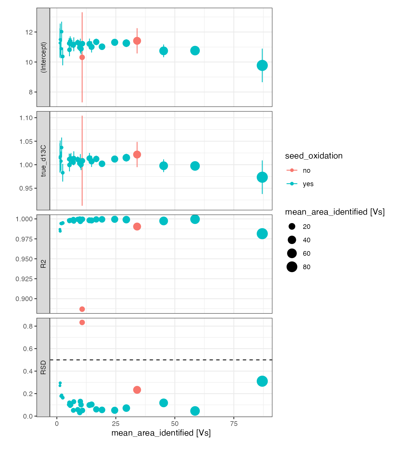
#> Info: there are no problematic calibrations

Coefficients

# look at coefficients and summary
stds_w_calibs %>% 
  # unnest calibration parameters
  iso_get_calibration_parameters(
    select_from_coefs = 
      c(term, estimate, SE = std.error, signif),
    select_from_summary = 
      c(fit_R2 = adj.r.squared, fit_RSD = sigma, residual_df = df.residual)) %>%
  arrange(term) %>% 
  knitr::kable(digits = 4)
#> Info: retrieving coefficient column(s) 'c(term, estimate, SE = std.error, signif)' for calibration
#> Info: retrieving summary column(s) 'c(fit_R2 = adj.r.squared, fit_RSD = sigma, residual_df = df.residual)' for calibration

Analysis	file_datetime	seed_oxidation	injection_volume	mean_area_identified	calib	calib_points	term	estimate	SE	signif	fit_R2	fit_RSD	residual_df
2034	2017-10-26 09:15:48	yes	0.5	1.316609	lm(d13C ~ true_d13C)	15	(Intercept)	11.2671	0.9756	*** (p < 0.001)	0.9870	0.2706	13
2041	2017-10-26 20:50:38	no	3.0	10.728124	lm(d13C ~ true_d13C)	15	(Intercept)	10.3123	3.0026	** (p < 0.01)	0.8869	0.8330	13
2047	2017-10-27 05:50:04	yes	3.0	13.834178	lm(d13C ~ true_d13C)	15	(Intercept)	11.2081	0.3546	*** (p < 0.001)	0.9983	0.0984	13
2093	2017-10-30 00:32:04	yes	0.5	2.032492	lm(d13C ~ true_d13C)	15	(Intercept)	12.0237	0.6659	*** (p < 0.001)	0.9941	0.1847	13
2099	2017-10-30 10:33:19	yes	0.5	2.497390	lm(d13C ~ true_d13C)	15	(Intercept)	10.3700	0.5911	*** (p < 0.001)	0.9949	0.1640	13
2114	2017-10-31 10:08:42	yes	1.5	5.675072	lm(d13C ~ true_d13C)	15	(Intercept)	11.3763	0.3359	*** (p < 0.001)	0.9984	0.0932	13
2035	2017-10-26 10:50:43	yes	1.5	5.356130	lm(d13C ~ true_d13C)	15	(Intercept)	10.8131	0.4285	*** (p < 0.001)	0.9974	0.1189	13
2096	2017-10-30 05:48:23	yes	1.5	8.855793	lm(d13C ~ true_d13C)	15	(Intercept)	11.2949	0.2081	*** (p < 0.001)	0.9994	0.0577	13
2100	2017-10-30 12:08:16	yes	1.5	9.864856	lm(d13C ~ true_d13C)	15	(Intercept)	11.1531	0.1618	*** (p < 0.001)	0.9996	0.0449	13
2115	2017-10-31 11:43:46	yes	3.0	10.838746	lm(d13C ~ true_d13C)	15	(Intercept)	11.2240	0.1824	*** (p < 0.001)	0.9995	0.0506	13
2139	2017-11-02 15:13:36	yes	1.0	29.445250	lm(d13C ~ true_d13C)	15	(Intercept)	11.2577	0.2570	*** (p < 0.001)	0.9991	0.0713	13
2032	2017-10-26 06:05:49	yes	1.5	5.237014	lm(d13C ~ true_d13C)	15	(Intercept)	11.2381	0.3698	*** (p < 0.001)	0.9981	0.1026	13
2036	2017-10-26 12:25:48	yes	3.0	10.256694	lm(d13C ~ true_d13C)	15	(Intercept)	10.8792	0.3646	*** (p < 0.001)	0.9981	0.1011	13
2045	2017-10-27 02:40:08	yes	0.5	1.786624	lm(d13C ~ true_d13C)	15	(Intercept)	10.8889	0.6412	*** (p < 0.001)	0.9943	0.1779	13
2056	2017-10-27 19:34:08	yes	1.5	14.721991	lm(d13C ~ true_d13C)	15	(Intercept)	11.0069	0.3724	*** (p < 0.001)	0.9981	0.1033	13
2075	2017-10-28 20:27:22	yes	1.5	6.011649	lm(d13C ~ true_d13C)	15	(Intercept)	11.2325	0.3605	*** (p < 0.001)	0.9982	0.1000	13
2097	2017-10-30 07:23:28	yes	3.0	16.704496	lm(d13C ~ true_d13C)	15	(Intercept)	11.3383	0.2171	*** (p < 0.001)	0.9993	0.0602	13
2101	2017-10-30 13:43:23	yes	3.0	19.140429	lm(d13C ~ true_d13C)	15	(Intercept)	11.0189	0.1998	*** (p < 0.001)	0.9994	0.0554	13
2136	2017-11-02 04:38:25	yes	0.5	9.705883	lm(d13C ~ true_d13C)	15	(Intercept)	10.9667	0.1148	*** (p < 0.001)	0.9998	0.0318	13
2140	2017-11-02 16:48:30	yes	2.0	58.566406	lm(d13C ~ true_d13C)	15	(Intercept)	10.7605	0.1660	*** (p < 0.001)	0.9996	0.0460	13
2033	2017-10-26 07:40:55	yes	3.0	9.967239	lm(d13C ~ true_d13C)	15	(Intercept)	11.0859	0.4703	*** (p < 0.001)	0.9969	0.1305	13
2046	2017-10-27 04:15:02	yes	1.5	7.189101	lm(d13C ~ true_d13C)	15	(Intercept)	11.1801	0.4632	*** (p < 0.001)	0.9970	0.1285	13
2060	2017-10-27 23:54:33	no	1.0	34.014913	lm(d13C ~ true_d13C)	15	(Intercept)	11.4129	0.8419	*** (p < 0.001)	0.9904	0.2336	13
2086	2017-10-29 13:58:06	yes	1.5	7.014310	lm(d13C ~ true_d13C)	15	(Intercept)	11.1096	0.1856	*** (p < 0.001)	0.9995	0.0515	13
2102	2017-10-30 15:18:16	yes	1.0	45.260003	lm(d13C ~ true_d13C)	15	(Intercept)	10.7432	0.4240	*** (p < 0.001)	0.9974	0.1176	13
2113	2017-10-31 08:33:47	yes	0.5	1.426427	lm(d13C ~ true_d13C)	15	(Intercept)	11.5001	1.0634	*** (p < 0.001)	0.9846	0.2950	13
2117	2017-10-31 14:53:43	yes	3.0	87.052984	lm(d13C ~ true_d13C)	15	(Intercept)	9.7739	1.1193	*** (p < 0.001)	0.9815	0.3105	13
2137	2017-11-02 06:13:18	yes	1.0	24.517030	lm(d13C ~ true_d13C)	15	(Intercept)	11.3123	0.1869	*** (p < 0.001)	0.9995	0.0519	13
2034	2017-10-26 09:15:48	yes	0.5	1.316609	lm(d13C ~ true_d13C)	15	true_d13C	1.0145	0.0311	*** (p < 0.001)	0.9870	0.2706	13
2041	2017-10-26 20:50:38	no	3.0	10.728124	lm(d13C ~ true_d13C)	15	true_d13C	1.0085	0.0958	*** (p < 0.001)	0.8869	0.8330	13
2047	2017-10-27 05:50:04	yes	3.0	13.834178	lm(d13C ~ true_d13C)	15	true_d13C	1.0137	0.0113	*** (p < 0.001)	0.9983	0.0984	13
2093	2017-10-30 00:32:04	yes	0.5	2.032492	lm(d13C ~ true_d13C)	15	true_d13C	1.0366	0.0213	*** (p < 0.001)	0.9941	0.1847	13
2099	2017-10-30 10:33:19	yes	0.5	2.497390	lm(d13C ~ true_d13C)	15	true_d13C	0.9830	0.0189	*** (p < 0.001)	0.9949	0.1640	13
2114	2017-10-31 10:08:42	yes	1.5	5.675072	lm(d13C ~ true_d13C)	15	true_d13C	1.0121	0.0107	*** (p < 0.001)	0.9984	0.0932	13
2035	2017-10-26 10:50:43	yes	1.5	5.356130	lm(d13C ~ true_d13C)	15	true_d13C	0.9995	0.0137	*** (p < 0.001)	0.9974	0.1189	13
2096	2017-10-30 05:48:23	yes	1.5	8.855793	lm(d13C ~ true_d13C)	15	true_d13C	1.0110	0.0066	*** (p < 0.001)	0.9994	0.0577	13
2100	2017-10-30 12:08:16	yes	1.5	9.864856	lm(d13C ~ true_d13C)	15	true_d13C	1.0066	0.0052	*** (p < 0.001)	0.9996	0.0449	13
2115	2017-10-31 11:43:46	yes	3.0	10.838746	lm(d13C ~ true_d13C)	15	true_d13C	1.0082	0.0058	*** (p < 0.001)	0.9995	0.0506	13
2139	2017-11-02 15:13:36	yes	1.0	29.445250	lm(d13C ~ true_d13C)	15	true_d13C	1.0149	0.0082	*** (p < 0.001)	0.9991	0.0713	13
2032	2017-10-26 06:05:49	yes	1.5	5.237014	lm(d13C ~ true_d13C)	15	true_d13C	1.0118	0.0118	*** (p < 0.001)	0.9981	0.1026	13
2036	2017-10-26 12:25:48	yes	3.0	10.256694	lm(d13C ~ true_d13C)	15	true_d13C	1.0001	0.0116	*** (p < 0.001)	0.9981	0.1011	13
2045	2017-10-27 02:40:08	yes	0.5	1.786624	lm(d13C ~ true_d13C)	15	true_d13C	1.0076	0.0205	*** (p < 0.001)	0.9943	0.1779	13
2056	2017-10-27 19:34:08	yes	1.5	14.721991	lm(d13C ~ true_d13C)	15	true_d13C	1.0071	0.0119	*** (p < 0.001)	0.9981	0.1033	13
2075	2017-10-28 20:27:22	yes	1.5	6.011649	lm(d13C ~ true_d13C)	15	true_d13C	1.0133	0.0115	*** (p < 0.001)	0.9982	0.1000	13
2097	2017-10-30 07:23:28	yes	3.0	16.704496	lm(d13C ~ true_d13C)	15	true_d13C	1.0123	0.0069	*** (p < 0.001)	0.9993	0.0602	13
2101	2017-10-30 13:43:23	yes	3.0	19.140429	lm(d13C ~ true_d13C)	15	true_d13C	1.0020	0.0064	*** (p < 0.001)	0.9994	0.0554	13
2136	2017-11-02 04:38:25	yes	0.5	9.705883	lm(d13C ~ true_d13C)	15	true_d13C	1.0030	0.0037	*** (p < 0.001)	0.9998	0.0318	13
2140	2017-11-02 16:48:30	yes	2.0	58.566406	lm(d13C ~ true_d13C)	15	true_d13C	0.9974	0.0053	*** (p < 0.001)	0.9996	0.0460	13
2033	2017-10-26 07:40:55	yes	3.0	9.967239	lm(d13C ~ true_d13C)	15	true_d13C	1.0076	0.0150	*** (p < 0.001)	0.9969	0.1305	13
2046	2017-10-27 04:15:02	yes	1.5	7.189101	lm(d13C ~ true_d13C)	15	true_d13C	1.0137	0.0148	*** (p < 0.001)	0.9970	0.1285	13
2060	2017-10-27 23:54:33	no	1.0	34.014913	lm(d13C ~ true_d13C)	15	true_d13C	1.0217	0.0269	*** (p < 0.001)	0.9904	0.2336	13
2086	2017-10-29 13:58:06	yes	1.5	7.014310	lm(d13C ~ true_d13C)	15	true_d13C	1.0049	0.0059	*** (p < 0.001)	0.9995	0.0515	13
2102	2017-10-30 15:18:16	yes	1.0	45.260003	lm(d13C ~ true_d13C)	15	true_d13C	0.9978	0.0135	*** (p < 0.001)	0.9974	0.1176	13
2113	2017-10-31 08:33:47	yes	0.5	1.426427	lm(d13C ~ true_d13C)	15	true_d13C	1.0174	0.0339	*** (p < 0.001)	0.9846	0.2950	13
2117	2017-10-31 14:53:43	yes	3.0	87.052984	lm(d13C ~ true_d13C)	15	true_d13C	0.9734	0.0357	*** (p < 0.001)	0.9815	0.3105	13
2137	2017-11-02 06:13:18	yes	1.0	24.517030	lm(d13C ~ true_d13C)	15	true_d13C	1.0120	0.0060	*** (p < 0.001)	0.9995	0.0519	13

# visualize the calibration coefficients
stds_w_calibs %>% 
  # plot calibration parameters
  iso_plot_calibration_parameters(
    # x-axis, could also be e.g. Analysis or file_datetime (also use date_breaks!)
    x = mean_area_identified,
    # aesthetics
    color = seed_oxidation, size = mean_area_identified,
    # highlight RSD threshold
    geom_hline(data = tibble(term = factor("RSD"), threshold = 0.5),
               mapping = aes(yintercept = threshold), linetype = 2)
  ) 

Residuals

stds_w_calibs %>% 
  # pull out all peak data to including residuals
  iso_get_calibration_data() %>% 
  # focus on standard peaks
  filter(is_std_peak) %>% 
  # calculate area deviation from mean
  iso_mutate_peak_table(
    group_by = Analysis,
    area_dev = iso_double_with_units((area44/mean(area44) - 1) * 100, "%")
  ) %>% 
  # visualize
  iso_plot_data(
    # x and y 
    x = compound, y = c(residual = resid, `area dev. from mean` = area_dev),
    # grouping and aesthetics
    group = paste(Analysis, calib), color = seed_oxidation, linetype = calib,
    # geoms
    lines = TRUE
  )
#> Info: retrieving all data
#> Info: mutating peak table grouped by 'Analysis', column(s) 'area_dev' added.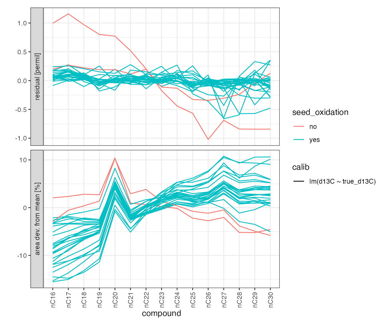

Global Calibration with all standards

Generate calibrations (*)

# define a global calibration across all standards
global_calibs <- 
  peak_table_w_stds %>%
  # remove (most) problematic peaks to speed up calibration calculations
  # note: could additionally remove unidentified peaks if they are of no interest
  iso_remove_problematic_peak_mappings(remove_unidentified = FALSE) %>% 
  # prepare for calibration (no grouping to go across all analyses)
  iso_prepare_for_calibration() %>% 
  # run different calibrations
  iso_generate_calibration(
    model = c(
      linear = lm(d13C ~ true_d13C),
      with_area = lm(d13C ~ true_d13C + area44),
      with_area_cross = lm(d13C ~ true_d13C * area44)
    ),
    # specify which peaks to include in the calibration, here:
    # - all std_peaks (this filter should always be included!)
    # - standard peaks between 5 and 100 Vs
    # - only analyses with seed oxidation (same as all the samples)
    use_in_calib = is_std_peak & area44 > iso_double_with_units(5, "Vs") & 
      area44 < iso_double_with_units(100, "Vs") & seed_oxidation == "yes"
  ) %>% 
  iso_remove_problematic_calibrations()
#> Info: removing 7 of 628 peak table entries because of problematic peak identifications (missing or ambiguous)
#> Info: preparing data for calibration by nesting the entire dataset
#> Info: generating calibration based on 3 models (linear = 'lm(d13C ~ true_d13C)', with_area = 'lm(d13C ~ true_d13C + area44)', with_area_cross = 'lm(d13C ~ true_d13C * area44)') for 1 data group(s) with standards filter 'is_std_peak & area44 > iso_double_with_units(5, "Vs") & area44 < ...'. Storing residuals in new column 'resid'. Storing calibration info in new column 'in_calib'.
#> Info: there are no problematic calibrations

Coefficients

# look at coefficients and summary
global_calibs %>% 
  # unnest calibration parameters
  iso_get_calibration_parameters(
    select_from_coefs = 
      c(term, estimate, SE = std.error, signif),
    select_from_summary = 
      c(fit_R2 = adj.r.squared, fit_RSD = sigma, residual_df = df.residual)) %>%
  arrange(term) %>% 
  knitr::kable(digits = 4)
#> Info: retrieving coefficient column(s) 'c(term, estimate, SE = std.error, signif)' for calibration
#> Info: retrieving summary column(s) 'c(fit_R2 = adj.r.squared, fit_RSD = sigma, residual_df = df.residual)' for calibration

calib	calib_points	term	estimate	SE	signif	fit_R2	fit_RSD	residual_df
linear	311	(Intercept)	11.0412	0.1113	*** (p < 0.001)	0.9962	0.139	309
with_area	311	(Intercept)	11.0931	0.1028	*** (p < 0.001)	0.9967	0.128	308
with_area_cross	311	(Intercept)	11.3321	0.1414	*** (p < 0.001)	0.9968	0.127	307
with_area	311	area44	-0.0027	0.0004	*** (p < 0.001)	0.9967	0.128	308
with_area_cross	311	area44	-0.0149	0.0050	** (p < 0.01)	0.9968	0.127	307
linear	311	true_d13C	1.0057	0.0036	*** (p < 0.001)	0.9962	0.139	309
with_area	311	true_d13C	1.0057	0.0033	*** (p < 0.001)	0.9967	0.128	308
with_area_cross	311	true_d13C	1.0133	0.0045	*** (p < 0.001)	0.9968	0.127	307
with_area_cross	311	true_d13C:area44	-0.0004	0.0002	* (p < 0.05)	0.9968	0.127	307

# visualize coefficients for the different global calibrations
global_calibs %>% iso_plot_calibration_parameters()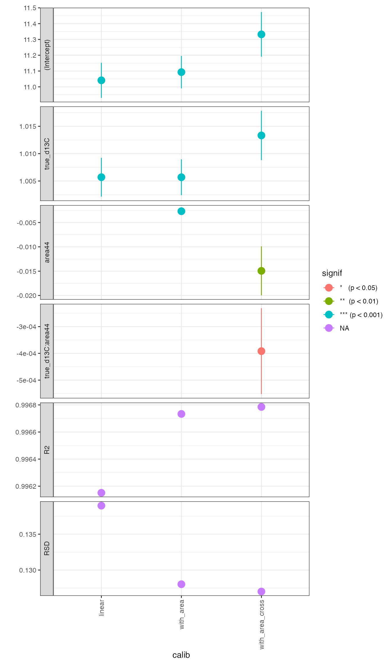

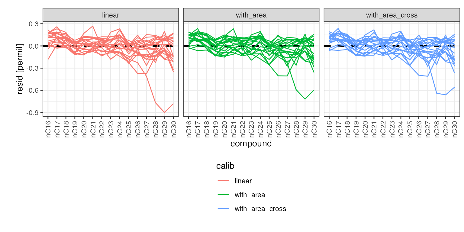
Residuals

global_calibs %>% 
  iso_plot_residuals(
    x = compound, group = paste(Analysis, calib), 
    points = FALSE, lines = TRUE,
    trendlines = FALSE, value_ranges = FALSE
  ) 

Apply global calibration (*)

# note that depending on the number of data points, this may take a while
# for faster calculations, chose calculate_error = FALSE
global_calibs_applied <- 
  global_calibs %>% 
  # which calibration to use? can include multiple if desired to see the result
  # in this case, the area conscious calibrations are not necessary
  filter(calib == "linear") %>% 
  # apply calibration indication what should be calcculated
  iso_apply_calibration(true_d13C, calculate_error = TRUE)
#> Info: applying calibration to infer 'true_d13C' for 1 data group(s) in 1 model(s); storing resulting value in new column 'true_d13C_pred' and estimated error in new column 'true_d13C_pred_se'. This may take a moment... finished.

# calibration ranges
global_calibs_with_ranges <-
  global_calibs_applied %>% 
  # evaluate calibration range for the measured area.Vs and predicted d13C
  iso_evaluate_calibration_range(area44, true_d13C_pred) 
#> Info: evaluating range for terms 'area44' and 'true_d13C_pred' in calibration for 1 data group(s) in 1 model(s); storing resulting summary for each data entry in new column 'in_range'.

# show calibration ranges
global_calibs_with_ranges %>% 
  iso_get_calibration_range() %>% 
  iso_remove_list_columns() %>% 
  knitr::kable(d = 2)
#> Info: retrieving all calibration range information for calibration

calib	calib_points	term	units	min	max
linear	311	area44	Vs	5.03	91.46
linear	311	true_d13C_pred	permil	-34.09	-25.94

# create calibrated peak table
peak_table_calibrated <- global_calibs_with_ranges %>% 
  iso_get_calibration_data()
#> Info: retrieving all data

Evaluation

Overview

# replicate earlier overview plot but now with the calibrated delta values
# and with a higlight of the calibration ranges and which points are in range
peak_table_calibrated %>% 
  # focus on identified peaks (comment out this line to see ALL peaks)
  filter(!is.na(compound)) %>% 
  # visualize with convenience function iso_plot_data
  iso_plot_data(
    # choose x and y (multiple y possible)
    x = area44, y = true_d13C_pred,
    # choose aesthetics
    color = in_range, shape = type, label = compound, size = 3,
    # decide what geoms to include
    points = TRUE
  ) %>% 
  # highlight calibration range
  iso_mark_calibration_range() +
  # further customize ggplot with a log scale x axis
  scale_x_log10() +
  # legend
  theme(legend.position = "bottom", legend.direction = "vertical")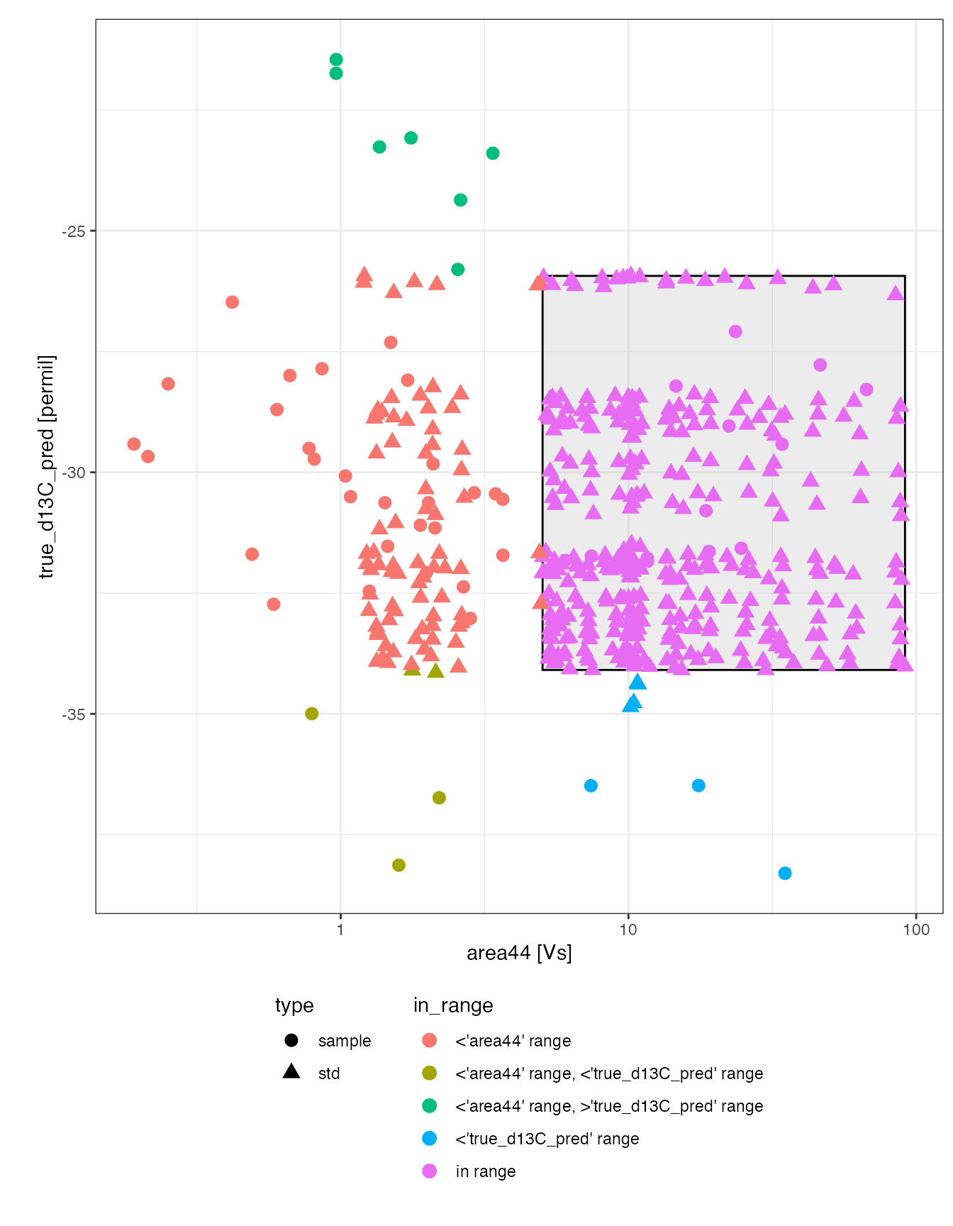

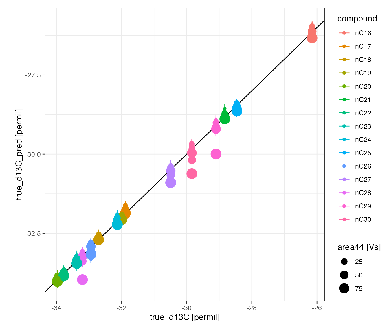
Standards

# visualize how standard line up after calibration
peak_table_calibrated %>% 
  # focus on peaks in calibration
  filter(in_calib) %>% 
  # visualize
  iso_plot_data(
    # x and y
    x = true_d13C, y = true_d13C_pred, y_error = true_d13C_pred_se,
    # aesthetics
    color = compound, size = area44,
    # geoms
    points = TRUE,
    # add 1:1 trendline
    geom_abline(slope = 1, intercept = 0)
  ) 

Data

Isotopic values

# Warning: data outside the calibration range MUST be taken with a
# grain of salt, especially at the low signal area/amplitude end
peak_table_calibrated %>% 
  # focus on samples
  filter(type == "sample") %>% 
  # focus on identified peaks (comment out this line to see ALL peaks)
  # if there's a lot of data, might need to hone in on a few at a time
  filter(!is.na(compound)) %>% 
  # visualize
  iso_plot_data(
    # x and y
    x = sample, y = true_d13C_pred, y_error = true_d13C_pred_se,
    # aesthetics
    color = in_range, size = rel_area, 
    # paneling
    panel = compound, panel_scales = "fixed",
    # geoms
    points = TRUE
  ) %>% 
  # mark calibration range (include optionally)
  iso_mark_calibration_range() +
  # color palette (here example of manual: www.google.com/search?q=color+picker)
  scale_color_manual(
    values = c("#984EA3", "#E41A1C", "#E41A1C", "#377EB8", "#4DAF4A")
  ) +
  # clarify size scale
  scale_size_continuous(breaks = c(0.01, 0.05, 0.1, 0.2, 0.3), 
                        labels = function(x) paste0(100*x, "%")) +
  # plot labels
  labs(x = NULL)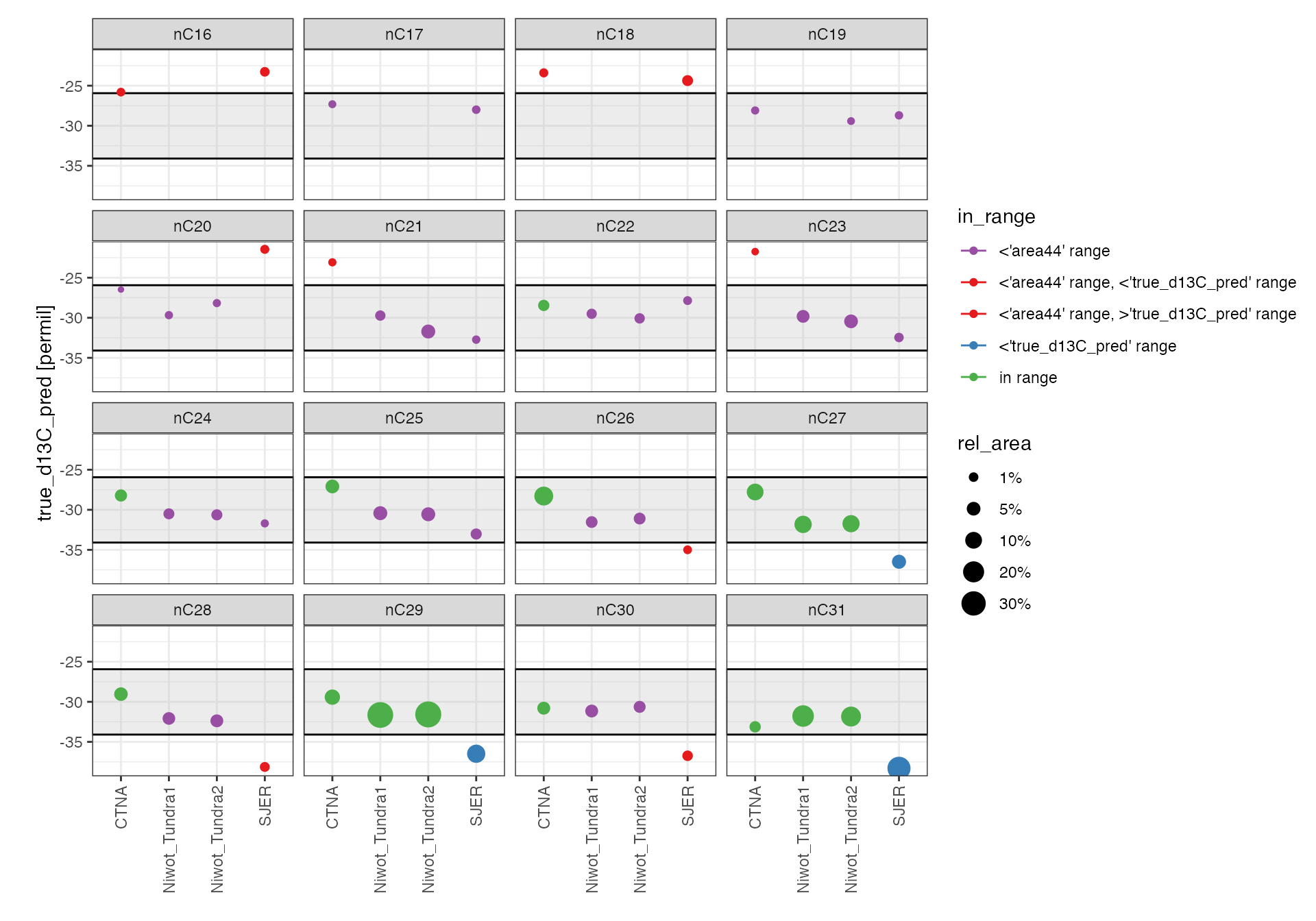

Relative abundances

# visualize relative abundances
peak_table_calibrated %>% 
  # focus on samples
  filter(type == "sample") %>% 
  # focus on identified peaks (comment out this line to see ALL peaks)
  #filter(!is.na(compound)) %>% 
  # visualize
  iso_plot_data(
    # x and y
    x = sample, y = rel_area,
    # aesthetics
    fill = compound,
    # barchart
    geom_bar(stat = "identity")
  ) +
  # scales
  scale_y_continuous(labels = function(x) paste0(100*x, "%"), expand = c(0, 0)) +
  # plot labels
  labs(x = NULL, y = "Relative abundance (by area)")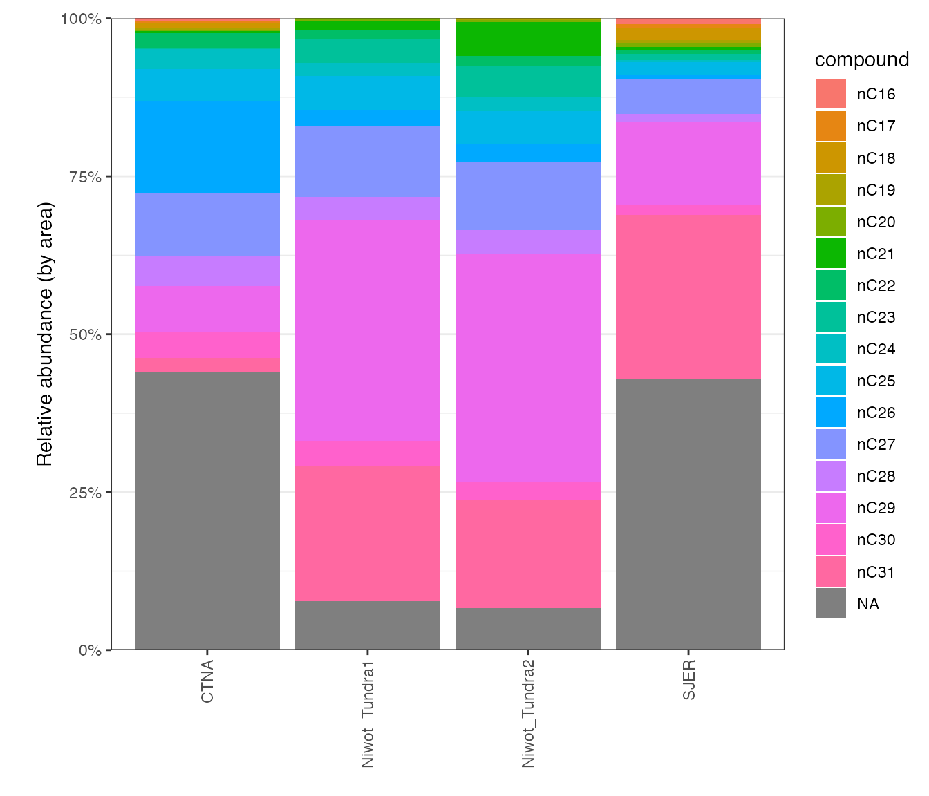

Summary

# generate data summary
peak_data <- 
  peak_table_calibrated %>% 
  # focus on identified peaks in the samples
  filter(type == "sample", !is.na(compound)) %>% 
  select(sample, compound, Analysis, 
         area44, true_d13C_pred, true_d13C_pred_se, in_range) %>% 
  arrange(sample, compound, Analysis) 

# summarize replicates
# this example data set does not contain any replicates but typically all
# analyses should in which case a statistical data summary can be useful
peak_data_summary <- 
  peak_data %>% 
  # here: only peaks within the area calibration range are included
  # you have to explicitly decide which peaks you trust if they are out of range
  filter(
    in_range %in% c("in range", "<'true_d13C_pred' range", ">'true_d13C_pred' range")
  ) %>% 
  # summarize for each sample and compound
  group_by(sample, compound) %>% 
  iso_summarize_data_table(area44, true_d13C_pred)

peak_data_summary %>% iso_make_units_explicit() %>% knitr::kable(d = 2)

sample	compound	n	area44 mean [Vs]	area44 sd	true_d13C_pred mean [permil]	true_d13C_pred sd
CTNA	nC22	1	10.53	NA	-28.46	NA
CTNA	nC24	1	14.63	NA	-28.22	NA
CTNA	nC25	1	23.56	NA	-27.09	NA
CTNA	nC26	1	67.20	NA	-28.29	NA
CTNA	nC27	1	46.40	NA	-27.78	NA
CTNA	nC28	1	22.36	NA	-29.04	NA
CTNA	nC29	1	34.20	NA	-29.42	NA
CTNA	nC30	1	18.60	NA	-30.80	NA
CTNA	nC31	1	10.82	NA	-33.12	NA
Niwot_Tundra1	nC27	1	6.04	NA	-31.82	NA
Niwot_Tundra1	nC29	1	19.08	NA	-31.64	NA
Niwot_Tundra1	nC31	1	11.63	NA	-31.78	NA
Niwot_Tundra2	nC27	1	7.44	NA	-31.73	NA
Niwot_Tundra2	nC29	1	24.67	NA	-31.57	NA
Niwot_Tundra2	nC31	1	11.65	NA	-31.84	NA
SJER	nC27	1	7.41	NA	-36.49	NA
SJER	nC29	1	17.53	NA	-36.48	NA
SJER	nC31	1	35.01	NA	-38.30	NA

Final

Final data processing and visualization usually depends on the type of data and the metadata available for contextualization (e.g. core depth, source organism, age, etc.). The relevant metadata can be added easily with iso_add_file_info() during the initial data load / file info procesing. Alternatively, just call iso_add_file_info() again at this later point or use dplyr’s left_join directly.

# @user: add final data processing and plot(s)

Export

# export the global calibration with all its information and data to Excel
peak_table_calibrated %>% 
  iso_export_calibration_to_excel(
    filepath = format(Sys.Date(), "%Y%m%d_gc_irms_example_carbon_export.xlsx"),
    # include data summary as an additional useful tab
    `data summary` = peak_data_summary
  )
#> Info: exporting calibrations into Excel '20211104_gc_irms_example_carbon_export.xlsx'...
#> Info: retrieving all data
#> Info: retrieving all coefficient information for calibration
#> Info: retrieving all summary information for calibration
#> Info: retrieving all calibration range information for calibration
#> Info: export complete, created tabs 'data summary', 'all data', 'calib coefs', 'calib summary' and 'calib range'.