Introduction
Isoprocessor supports several plotting and data conversion functions specifically for continuous flow data. This vignette shows some of the functionality for continuous flow files read by the isoreader package (see the corresponding vignette for details on data retrieval, storage and export).
# load isoreader and isoprocessor packages
library(isoreader)
library(isoprocessor)
Reading files
# read a few of the continuous flow examples provided with isoreader
cf_files <-
  iso_read_continuous_flow(
    iso_get_reader_example("continuous_flow_example.cf"),
    iso_get_reader_example("continuous_flow_example.iarc"),
    iso_get_reader_example("continuous_flow_example.dxf")
  )
#> Info: preparing to read 3 data files (all will be cached)...
#> Info: reading file 'continuous_flow_example.cf' with '.cf' reader...
#> Info: reading file 'continuous_flow_example.iarc' with '.iarc' reader...
#> Warning: caught error - 'rhdf5' package is required to read .iarc, please r...
#> Info: reading file 'continuous_flow_example.dxf' with '.dxf' reader...
#> Info: finished reading 3 files in 5.62 secs
#> Warning: encountered 1 problem.
#> # | FILE                         | PROBLEM | OCCURRED IN        | DETAILS
#> 1 | continuous_flow_example.iarc | error   | iso_read_flow_iarc | 'rhdf5' pac...
#> Use iso_get_problems(...) for more details.
Chromatograms
Plotting the raw data (i.e. the mass chromatograms) can be done either with the generic iso_plot_raw_data() function for a simple plot with default parameters, or directly using the continuous flow specific iso_plot_continuous_flow() (recommended), which can be highly customized. Note that the following plot shows the data from all files in their originally recorded signal intensity units. For examples of how to convert to a common unit, see the section on Signal conversion further down.
iso_plot_continuous_flow_data(cf_files)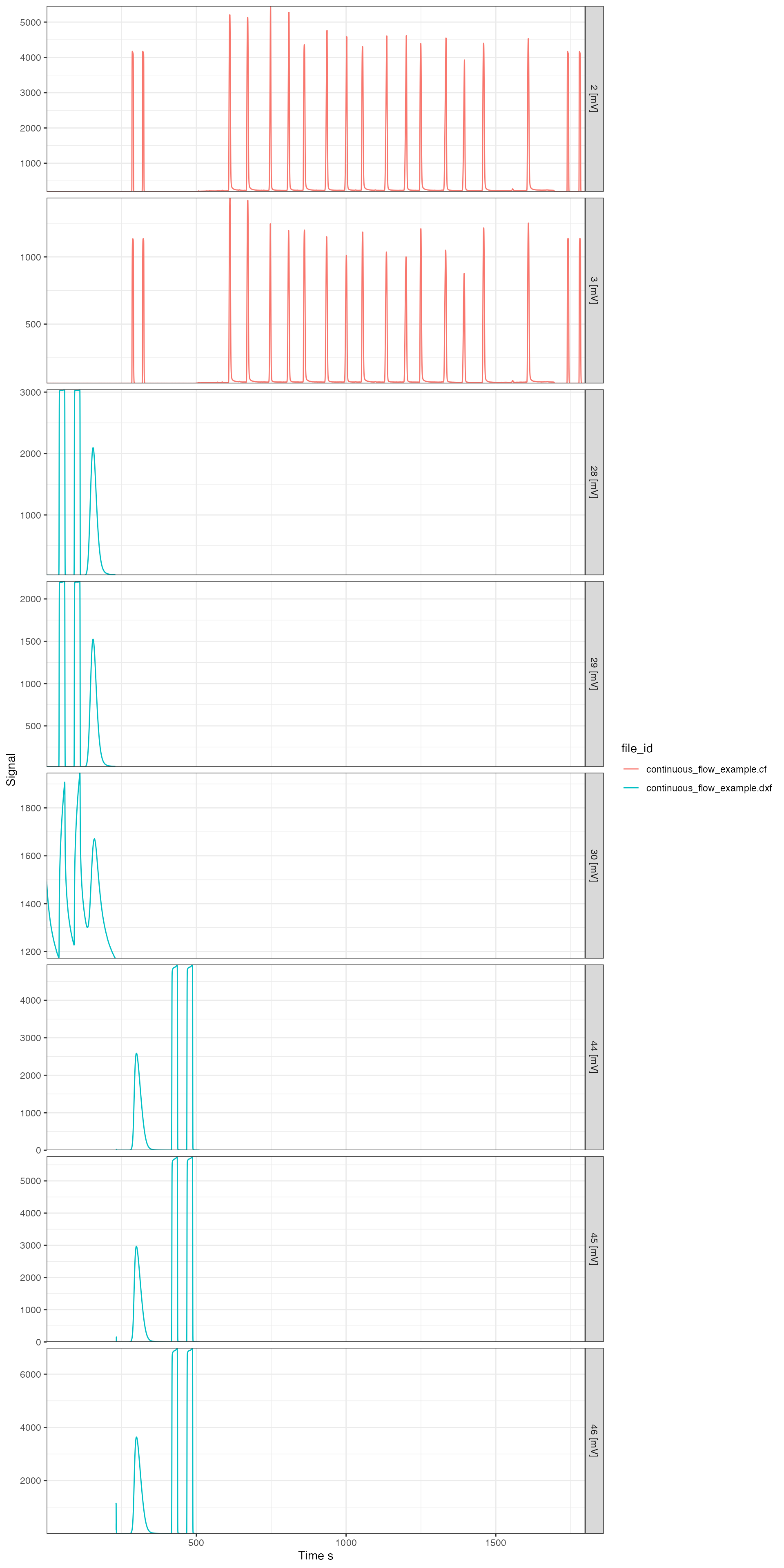
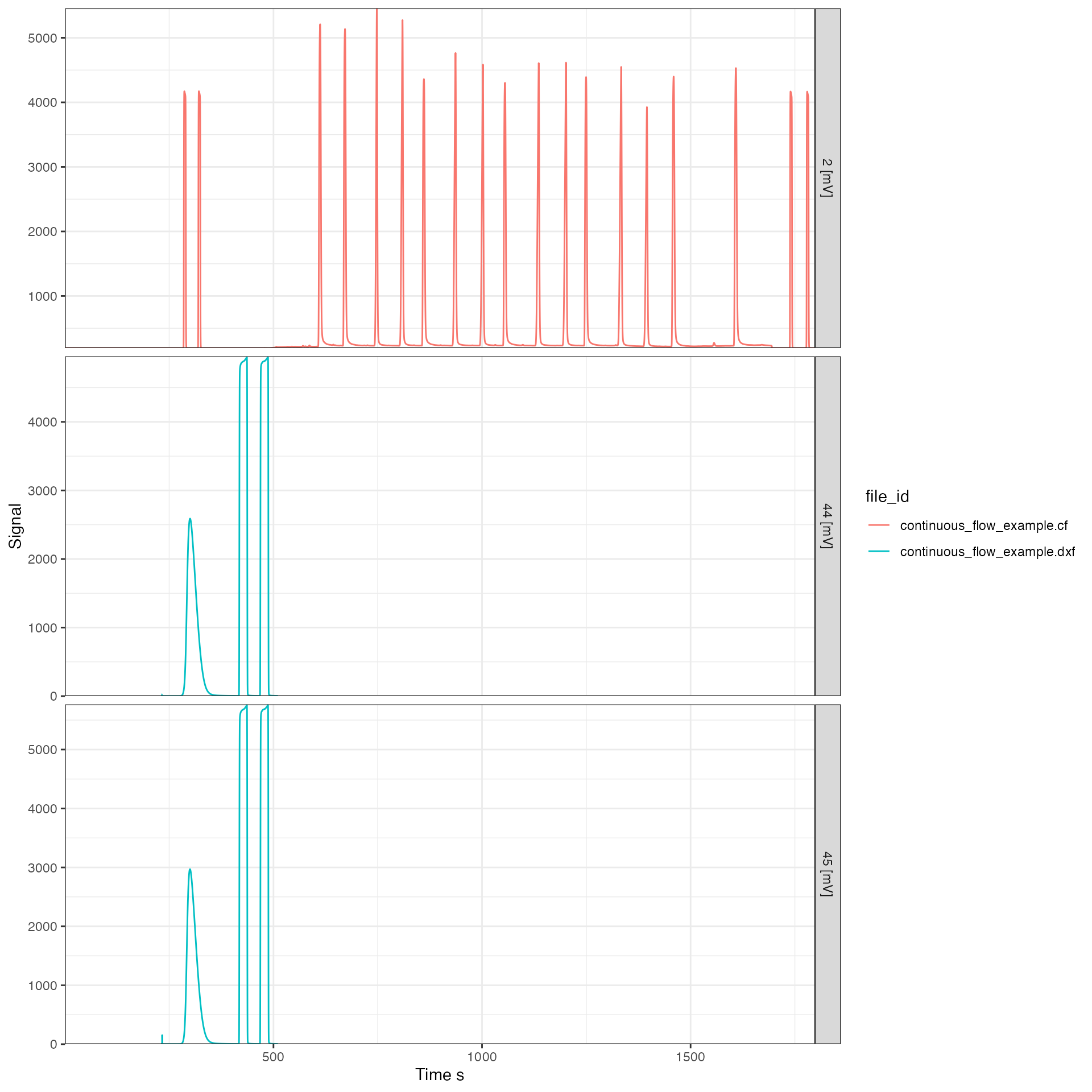
All customization options are described in the function help (?iso_plot_continuous_flow_data) and include, for example, plotting only a specific subset of masses (which will omit data from files that don’t include this mass):
# plot just masses 2, 44 and 45
iso_plot_continuous_flow_data(
  cf_files,
  data = c("2", "44", "45")
)
Peak Table
Continuous flow data is usually interpreted in the context of the individiual peaks in the chromatogram. For this purpose, isoprocessor provides several functions to set the peak table including iso_set_peak_table() (set a peak table manually), iso_set_peak_table_from_vendor_data_table() (use the data table precomputed by the vendor software and extracted from the data files by isoreader), and iso_find_peaks() (find peaks de novo from the raw chromatographic data). The latter is not yet implemented but coming soon. Here we provide the example of setting the peak table from Isodat-computed data.
# this is a convenience function to set peak table from isodat data table, it
# provides detailed information on the information copied to the peak table
cf_files <- iso_set_peak_table_from_isodat_vendor_data_table(cf_files)
#> Info: setting peak table for 3 file(s) from vendor data table with the following renames:
#> - for 1 file(s): 'Nr.'->'peak_nr', 'Is Ref.?'->'is_ref', 'Start'->'rt_start', 'Rt'->'rt', 'End'->'rt_end', 'Ampl 2'->'amp2', 'Ampl 3'->'amp3', 'BGD 2'->'bgrd2_start', 'BGD 3'->'bgrd3_start', 'BGD 2'->'bgrd2_end', 'BGD 3'->'bgrd3_end', 'rIntensity 2'->'area2', 'rIntensity 3'->'area3', 'rR 3H2/2H2'->'r3/2', 'rd 3H2/2H2'->'rd3/2', 'd 3H2/2H2'->'d3/2', 'd 2H/1H'->'d2H', 'AT% 2H/1H'->'at2H'
#> - for 1 file(s): 'Nr.'->'peak_nr', 'Is Ref.?'->'is_ref', 'Start'->'rt_start', 'Rt'->'rt', 'End'->'rt_end', 'Ampl 28'->'amp28', 'Ampl 29'->'amp29', 'Ampl 30'->'amp30', 'Ampl 44'->'amp44', 'Ampl 45'->'amp45', 'Ampl 46'->'amp46', 'BGD 28'->'bgrd28_start', 'BGD 29'->'bgrd29_start', 'BGD 30'->'bgrd30_start', 'BGD 44'->'bgrd44_start', 'BGD 45'->'bgrd45_start', 'BGD 46'->'bgrd46_start', 'BGD 28'->'bgrd28_end', 'BGD 29'->'bgrd29_end', 'BGD 30'->'bgrd30_end', 'BGD 44'->'bgrd44_end', 'BGD 45'->'bgrd45_end', 'BGD 46'->'bgrd46_end', 'rIntensity 28'->'area28', 'rIntensity 29'->'area29', 'rIntensity 30'->'area30', 'rIntensity 44'->'area44', 'rIntensity 45'->'area45', 'rIntensity 46'->'area46', 'rR 29N2/28N2'->'r29/28', 'rR 45CO2/44CO2'->'r45/44', 'rR 46CO2/44CO2'->'r46/44', 'rd 29N2/28N2'->'rd29/28', 'rd 45CO2/44CO2'->'rd45/44', 'rd 46CO2/44CO2'->'rd46/44', 'd 29N2/28N2'->'d29/28', 'd 45CO2/44CO2'->'d45/44', 'd 46CO2/44CO2'->'d46/44', 'd 15N/14N'->'d15N', 'd 13C/12C'->'d13C', 'd 18O/16O'->'d18O', 'd 17O/16O'->'d17O', 'AT% 15N/14N'->'at15N', 'AT% 13C/12C'->'at13C', 'AT% 18O/16O'->'at18O'

# display the resulting peak table now stored in the cf_files for the first file
cf_files[1] %>% iso_get_peak_table() %>% rmarkdown::paged_table()
#> Info: aggregating peak table from 1 data file(s)
Peak Labels
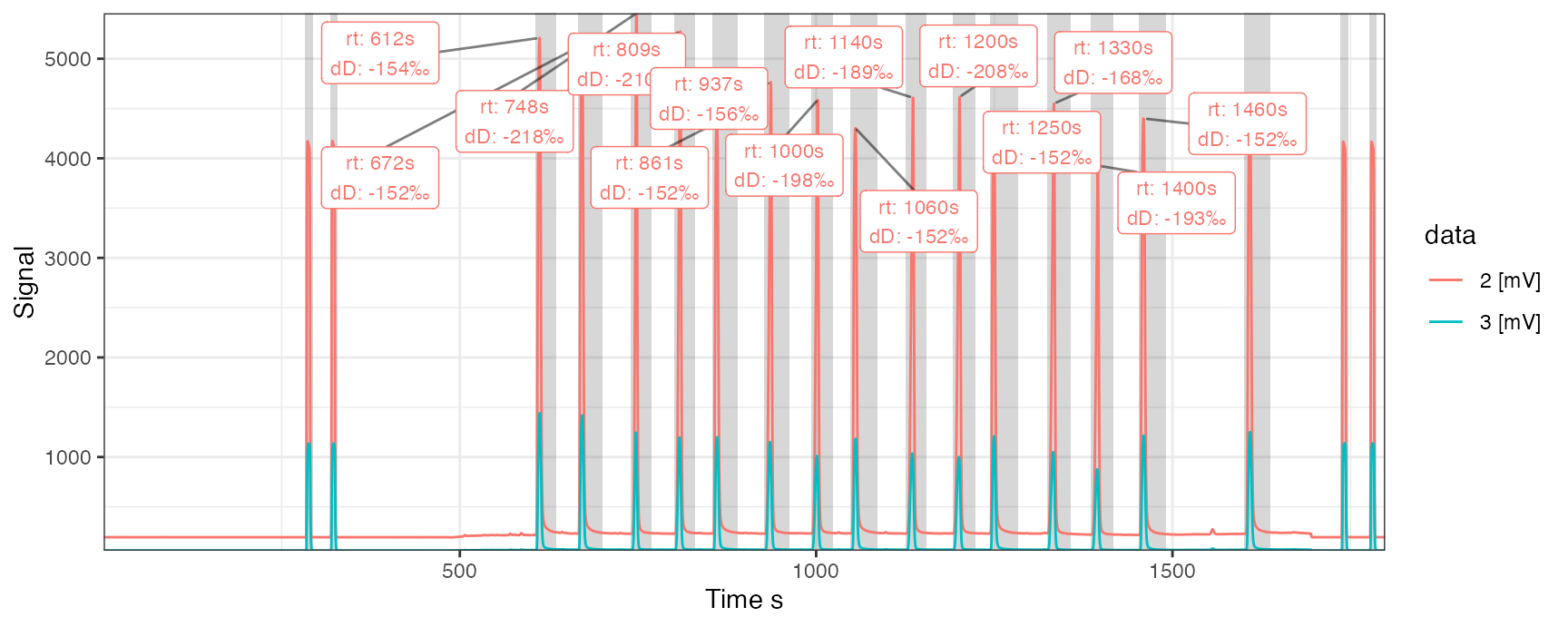
Since peak information is often key for interpretating chromatograms, the iso_plot_continuous_flow_data function also provides a suite of peak data integration parameters that make it easy to highlight peaks in the chromatogram and label them with any number of desired information. Now that the collection of cf_files has peak table information stored within, it is easy to make use of these for visualization.
iso_plot_continuous_flow_data(
  cf_files,
  # select which data to plot and how to plot it
  data = c("2", "3"), color = data, panel = NULL,
  # specify what to highlight about the peaks (here: bounds, ret. time and dD)
  peak_bounds = TRUE,
  peak_label = iso_format(rt, dD = d2H, signif = 3),
  peak_label_options = list(size = 3),
  # specify which labels to display (only the 2 trace, between 500 and 1500s)
  peak_label_filter = data == "2 [mV]" & dplyr::between(time.s, 500, 1500)
)
Isotope ratios
Raw data typically only includes ion signals but isotope ratios are often needed to calculate and visualize the data. For this purpose, isoreader provides a dynamic ratio calculation function (iso_calculate_ratios()) that accepts any combination of masses, here demonstrated for the standard CO2 ratios \(\frac{46}{44}\) and \(\frac{45}{44}\). Additionally, the following example demonstrates how the filter parameter can be used to exclude plotting artifacts (here e.g. the extreme ratio values seen right after the magnet jump). Notice how the ratios calculated from current intensities are close to 0 (as the real ratios likely are) whereas those calculated from voltages are close to 1 (due to the so chosen, different resistors in the detector circuit). See the section on Signal conversion further down on how to scale to uniform intensity units to address this comparison obstacle.
cf_files <-
  cf_files %>%
  # calculate 46/44 and 45/44 ratios
  iso_calculate_ratios(ratios = c("46/44", "45/44"))
#> Info: calculating ratio(s) in 2 data file(s): r46/44, r45/44

iso_plot_continuous_flow_data(
  cf_files,
  # visualize ratios along with main ion
  data = c("44", "45/44", "46/44"),
  # plot all masses but ratios only 0 to 2 to omit peak jump artifacts
  filter = category == "mass" | dplyr::between(value, 0, 2)
) + ggplot2::expand_limits(y = -0.3)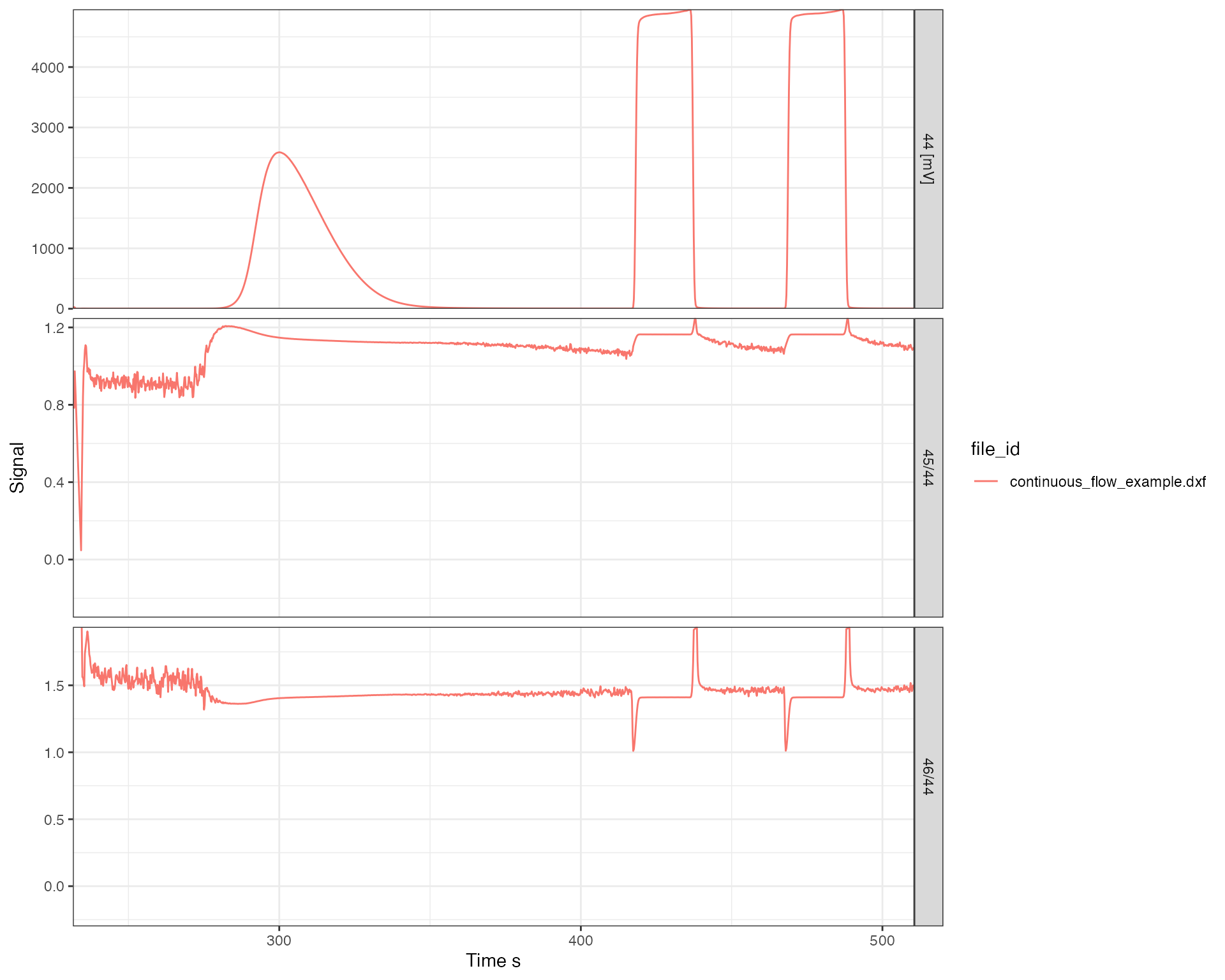
Time conversion
Most continuous flow data is reported in time units of seconds but this is not always the most useful unit. Isoreader provides easy time scaling functionality that will work for all standard time units (minutes, hours, days, etc.) regardless of which time units individual isofiles were initially recorded in.
# convert to minutes
cf_files <- iso_convert_time(cf_files, to = "minutes")
#> Info: converting time to 'minutes' for 3 continuous flow data file(s)

# plot masses 2 and 3
iso_plot_continuous_flow_data(cf_files, data = c(2, 3))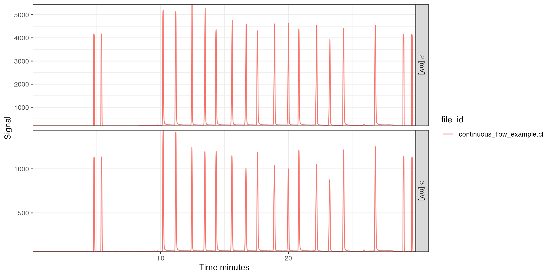
In this context, another useful customization option of the plotting function is the option to select a specific time window (in any time units, regardless of what is plotted), and the possibility to adjust plot aesthetics such as color, linetype, and paneling:
cf_files %>%
  # calculate 3/2 ratio on the file
  iso_calculate_ratios("3/2") %>%
  iso_plot_continuous_flow_data(
    # replot masses 2 and 3 together with the ratio for a specific time window
    data = c("2", "3", "3/2"),
    time_interval = c(10, 13),
    time_interval_units = "minutes",
    # adjust plot aesthetics to panel by masses vs. ratios and color by traces
    panel = category,
    color = data,
    # add peak labels
    peak_label = iso_format(RT = rt, A = amp2),
    peak_label_filter = data == "2 [mV]",
    peak_label_options = list(size = 4)
  )
#> Info: calculating ratio(s) in 2 data file(s): r3/2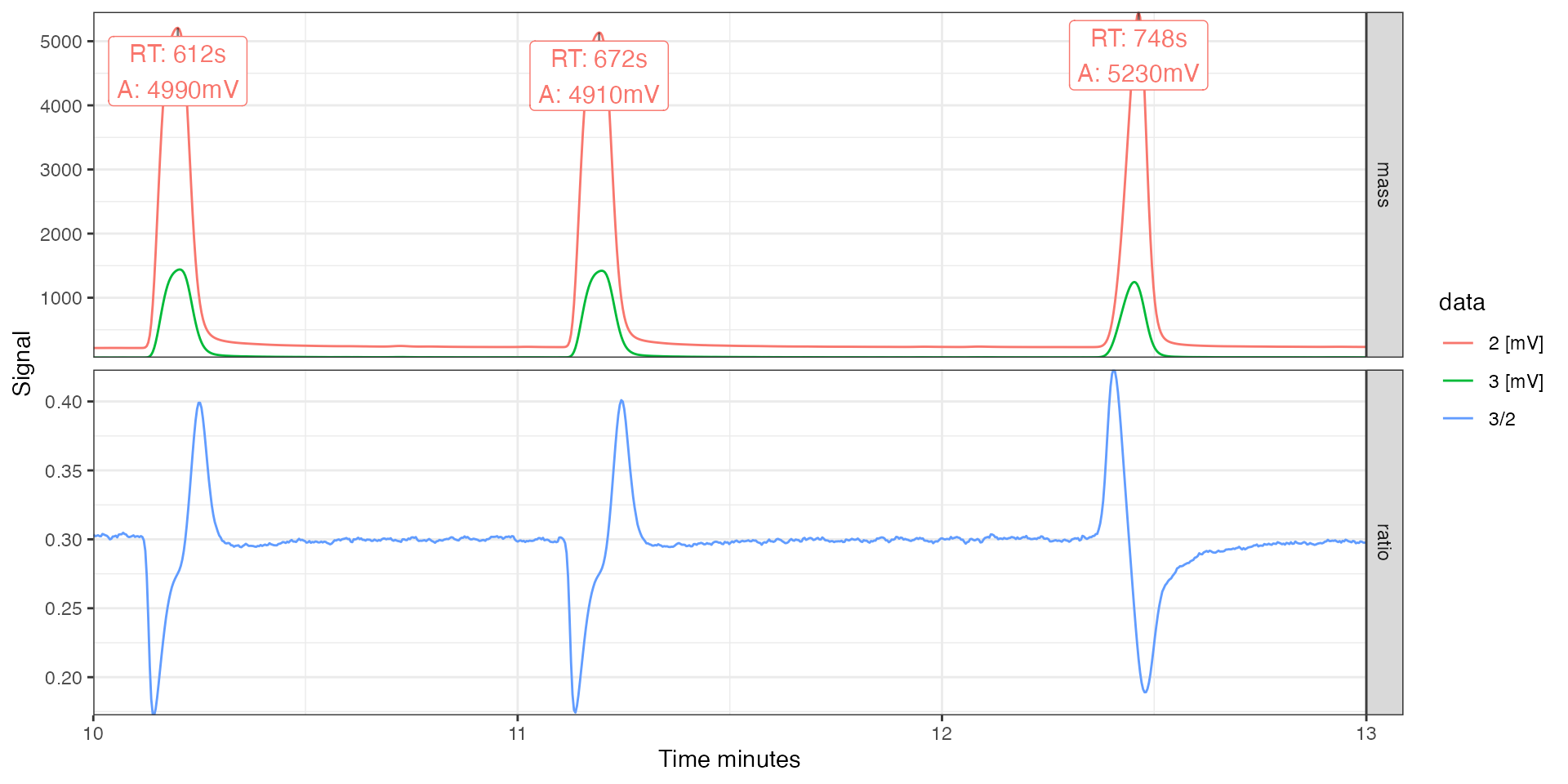
Signal conversion
Likewise, isoreader can convert between different signal units. This is particularly useful for comparing data files from different mass specs that record signals differentally. The earlier plot of mass 44 illustrated this scenario where some data was recorded in mV and some in nA. Voltages and currents can be scaled within each unit without restriction and with any valid SI prefix (e.g. from mV to V or nA to pA), however, for conversion from voltage to current or vice-versa, the appropriate resistor values need to be provided or be available from the data files themselves. The following is an example of scaling from voltage to current with the resistor values automatically read from the original data files (see file information section for details). Notice how the mass 44 signal is now in the same units for all files and the ratios are on comparable scales because they are calculated from the same unit intensities:
cf_files %>%
  # convert all signals to nano ampere
  iso_convert_signals(to = "nA") %>%
  # re-calculate ratios with the new unuts
  iso_calculate_ratios(ratios = c("46/44", "45/44")) %>%
  # re-plot same plot as earlier
  iso_plot_continuous_flow_data(
    data = c("44", "45/44", "46/44"),
    filter =
      category == "mass" |
      (data == "45/44" & dplyr::between(value, 0.005, 0.03)) |
      (data == "46/44" & dplyr::between(value, 0, 0.012))
  )
#> Info: converting signals to 'nA' for 3 data file(s) with automatic resistor values from individual iso_files (if needed for conversion)
#> Warning: encountered 1 problem(s) during signal conversion (1 total problems):
#> # A tibble: 1 × 4
#>   file_id                      type  func               details
#>   <chr>                        <chr> <chr>              <chr>
#> 1 continuous_flow_example.iarc error iso_read_flow_iarc 'rhdf5' package is requ…
#> Info: calculating ratio(s) in 2 data file(s): r46/44, r45/44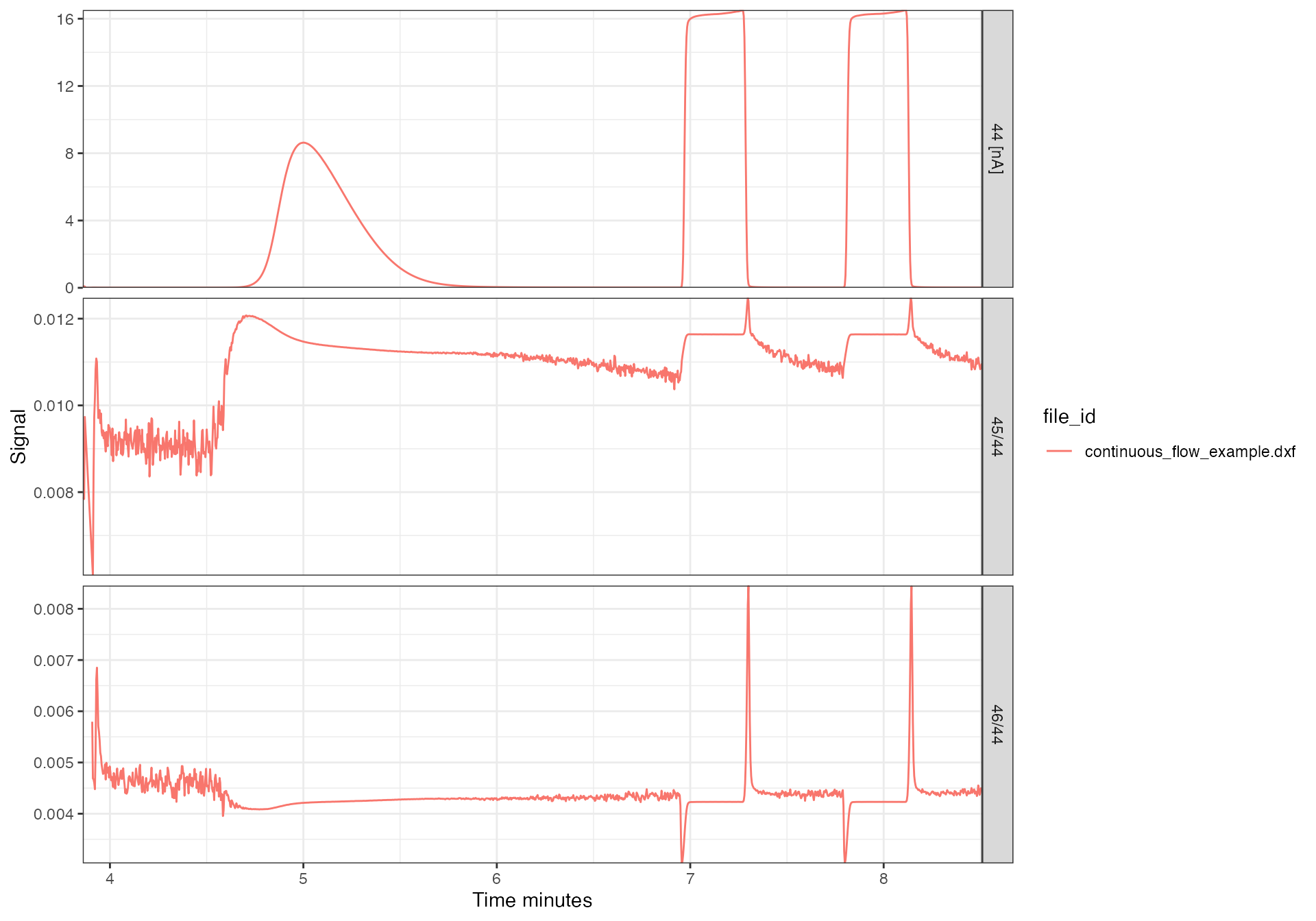
Plot styling
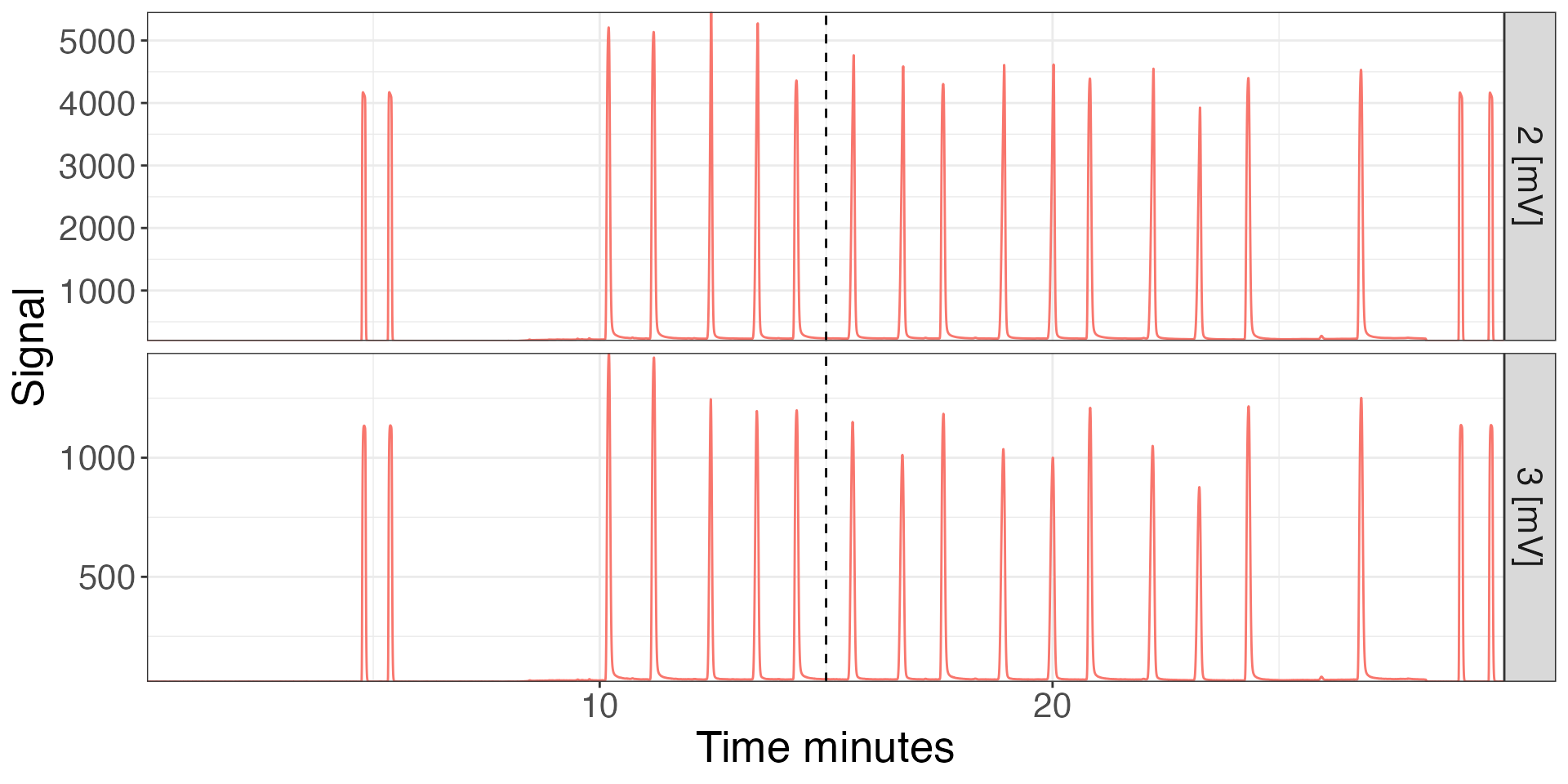
Since all isoreader plots are standard ggplot objects, they can be modified with any ggplot commands. For example to modify the themes:
library(ggplot2)
# replot
iso_plot_continuous_flow_data(cf_files, data = c(2,3)) +
  # add vertical dashed line (ggplot functionality)
  geom_vline(xintercept = 15, linetype = 2) +
  # modify plot styling (ggplot functionality)
  theme(text = element_text(size = 20),
        legend.position = "none")